37  The Eval Platform: A Number Someone Will Trust

This chapter runs the measurement-infrastructure family at interview depth, on the design a 2026 senior loop asks more than any other after retrieval: an evaluation platform. We take the prompt as the interviewer gives it and work the seven moves from Chapter 33 in order, then close with the interviewer probes and the family skeleton that transfers the design to guardrail, audit, and A/B siblings. The family’s defining move, recall from Section 33.2, is that the evidence plane is promoted to the product: the deliverable is a number, and the design question is whether anyone should trust it.

37.1 Scoping the eval platform

The prompt, as the interviewer says it: “Design an evaluation platform for our engineering org. Dozens of teams ship changes to LLM features every day, we keep shipping quality regressions we only hear about from user complaints, and I want the thing that catches a bad change before it merges, tells us whether quality is holding in production, and produces numbers we trust enough to block a launch on.” It names no metric, no owner of “correct,” no latency budget. The gaps are the interview.

Three clarifiers fork the architecture. The first is the family fork, and a senior asks it first: who owns ground truth? If “correct” is defined centrally, one global metric could work; but across dozens of teams a support bot, a code assistant, and a summarizer share no definition of good, so ground truth is per-team. That single answer turns datasets and judges into versioned artifacts keyed by team, and it tells us what the platform owns — the machinery, never the bar. The second: does the gate block a merge, or only report? Blocking pre-merge makes latency and stability first-class (a false block is an expensive insult to an engineer with a correct change), which pushes the thorough, slow evaluation out of the merge path. The third: are humans in the labeling loop continuously? They must be, because a judge is an instrument that drifts; that answer makes human labels the platform’s dominant recurring cost, a fact move 2 will price. Out of scope, said aloud: one universal quality score, a judge sitting in the request hot path, and grading any construct the platform cannot get a team to define.

Table 37.1: The eval platform restated with numbers, each row naming the decision its answer forces.

Requirement	Target (illustrative)	Why it forks the design
Teams served	~40, each with its own “good”	ground truth is per-team, so datasets and judges are versioned artifacts, not one metric
Pre-merge gate latency	p95 under 5 min	a small pinned golden set runs in CI; the full suite runs nightly, out of band
Gate decision rule	block regressions without flaking	paired candidate-minus-baseline delta with a confidence interval, not an absolute bar
Judge trust bar	{\kappa \ge 0.60} vs adjudicated humans	the judge is a calibrated instrument; a prompt or model change re-opens calibration
Online quality	sample prod, score asynchronously	the judge never sits in the request path
Out of scope	universal quality score; in-path judging	stated so the design is not blamed for omitting it

37.2 The numbers first

Numbers before boxes. The measurement family has one classic numeric trap, and it is the analogue of the KV-heads trap in serving: gate on Cohen’s {\kappa}, not raw agreement. A judge that agrees with humans 90 percent of the time sounds calibrated until you notice the set is 90 percent pass — a judge that says “pass” to everything scores the same and has measured nothing. We import the calculator that says so, reusing Chapter 22’s cohen_kappa (the owner of judge calibration, Section 22.3) rather than rebuilding it, alongside the back-of-envelope toolkit from Chapter 33.

import importlib.util
import sys
from pathlib import Path


def load_chapter(chapter: str, name: str):
    """Import a committed chapter's tangled module under an explicit name."""
    spec = importlib.util.spec_from_file_location(name, Path("code") / chapter / "_generated.py")
    module = importlib.util.module_from_spec(spec)
    sys.modules[name] = module
    spec.loader.exec_module(module)
    return module


sd = load_chapter("ch33", "ch33_sd")     # the back-of-envelope toolkit from Chapter 33
ev = load_chapter("ch22", "ch22_eval")   # Cohen's kappa from Chapter 22

human = ["pass"] * 85 + ["fail"] * 15    # a set that is 85% genuine pass
lazy = ["pass"] * 100                     # the laziest judge: always "pass"
raw = sum(h == j for h, j in zip(human, lazy)) / len(human)
print(f"always-pass judge on an 85%-pass set:")
print(f"  raw agreement = {raw:.2f}   Cohen's kappa = {ev.cohen_kappa(human, lazy):+.2f}")
print(f"  a trustworthy judge must clear kappa >= 0.60")

always-pass judge on an 85%-pass set:
  raw agreement = 0.85   Cohen's kappa = +0.00
  a trustworthy judge must clear kappa >= 0.60

Eighty-five percent agreement, kappa exactly zero: the raw number was lying and kappa says so in one figure. That is the sentence to say aloud in move 2 — the same way a serving candidate says “GQA caches KV heads, not query heads.” Next, the money. A judge grade is one cheap model call; we price the tiers with the toolkit’s cost_per_query.

judge = sd.TokenPrice(input_per_million=3.00, output_per_million=15.00)
per_grade = sd.cost_per_query(1_500, 120, judge)     # grade one (prompt, answer) pair
ci_items, nightly_items, online_per_day, merges = 300, 5_000, 20_000, 20
sme_rate, sme_hours = 60.0, 6.0                        # loaded SME cost per hour, illustrative

ci_run = per_grade * ci_items
nightly = per_grade * nightly_items * 0.5             # Batch API, ~50% off, latency-tolerant
online = per_grade * online_per_day
human_day = sme_rate * sme_hours
compute_day = ci_run * merges + nightly + online
print(f"one judge grade            : ${per_grade:.4f}")
print(f"per-merge CI run (300)     : ${ci_run:6.2f}")
print(f"nightly full suite (Batch) : ${nightly:6.2f}")
print(f"online sampling / day      : ${online:6.2f}")
print(f"all compute / day          : ${compute_day:6.2f}")
print(f"human calibration / day    : ${human_day:6.2f}   ({human_day / compute_day:.1f}x all compute)")

one judge grade            : $0.0063
per-merge CI run (300)     : $  1.89
nightly full suite (Batch) : $ 15.75
online sampling / day      : $126.00
all compute / day          : $179.55
human calibration / day    : $360.00   (2.0x all compute)

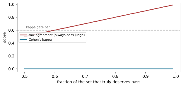
The anchor numbers, six of them, each one sentence of narration: a grade is two-thirds of a cent; a blocking CI run costs under two dollars because it grades only a small pinned set; the nightly full suite is cheap because it runs on the Batch API at roughly half price where a same-day answer is fine; online sampling is a hundred-odd dollars a day; and human calibration alone costs about twice the entire day’s compute. That last number is the design’s center of gravity — the platform’s scarce resource is not GPUs, it is human labels — and saying so reframes every later decision. The trap avoided aloud stays kappa, not agreement. Figure 37.1 draws why the trap is not a corner case but a curve.

import numpy as np
import matplotlib.pyplot as plt

rng = np.linspace(0.50, 0.99, 60)
raw_curve, kappa_curve = [], []
for p in rng:
    npass = int(round(p * 400))
    hum = ["pass"] * npass + ["fail"] * (400 - npass)
    alw = ["pass"] * 400
    raw_curve.append(sum(a == b for a, b in zip(hum, alw)) / 400)
    kappa_curve.append(ev.cohen_kappa(hum, alw))

fig, ax = plt.subplots(figsize=(6.6, 3.2))
ax.plot(rng, raw_curve, color="#b13f3f", lw=2, label="raw agreement (always-pass judge)")
ax.plot(rng, kappa_curve, color="#2a7f9e", lw=2, label="Cohen's kappa")
ax.axhline(0.60, ls="--", color="0.4")
ax.text(0.505, 0.63, "kappa gate bar", fontsize=8, color="0.4")
ax.set_xlabel("fraction of the set that truly deserves pass")
ax.set_ylabel("score")
ax.set_ylim(-0.05, 1.02)
ax.legend(loc="center left", fontsize=8)
fig.tight_layout()
plt.show()

Figure 37.1: Why does a high-agreement judge tell you nothing? As the pass rate skews, an always-pass judge’s raw agreement climbs toward one while its kappa stays pinned at zero. The gate must read the line that does not lie.

NoteLandscape 2026 — the constants in this study

The judge prices ($3.00 and $15.00 per million tokens, reused from Chapter 33), the $60/hour loaded reviewer rate, the {\kappa \ge 0.60} bar, the 5-minute gate budget, and the 7 percent judge-error rate used below are illustrative teaching constants for round arithmetic. Kappa thresholds in particular are conventions, not laws; a real bar is derived from the harm of a false promotion versus a false block. Verify live: your provider’s pricing and Batch discount, your own human-label costs, and your measured judge confusion matrix. Checked 2026-07-20.

37.3 The contract and the two-loop skeleton

The caller-visible contract is three verbs. submit(candidate, dataset_version, judge_version) returns a verdict, the blocking reasons, and the full evidence packet; calibrate(judge_version, human_labels) returns the judge’s kappa, failure-recall, and position-flip rate; sample_online(release, rate) scores production traffic out of band. The service levels follow the requirements table: the blocking gate clears p95 under five minutes, every verdict is reproducible from its pinned dataset and judge versions plus a seed, and the judge holds {\kappa \ge 0.60} or the gate refuses to trust it. The success metrics are the platform’s own: caught-regression rate, escaped-regression rate (regressions that reached production the gate missed), and gate flake rate — because a gate nobody trusts is worse than no gate, since it trains engineers to override it.

Now the boxes, and the skeleton is the family’s signature: two loops that never merge. Figure 37.2 draws them.

flowchart TB
    subgraph CUR ["dataset-curation loop — what does 'good' mean?"]
        TR["prod traces"] -. "sample · redact · dedupe" .-> REV["SME review"]
        DES["designed coverage<br/>threats · slices"] --> REV
        REV --> DS[("versioned eval set<br/>silver → gold → mined")]
    end
    subgraph CAL ["judge-calibration loop — can the instrument measure it?"]
        HL["human labels"] --> KAP["kappa · fail-recall<br/>flip-rate · slice tests"]
        KAP --> JG[("versioned judge<br/>prompt · model · parser")]
    end
    CAND["candidate build"] --> GATE{"paired gate<br/>candidate − baseline + CI"}
    DS --> GATE
    JG --> GATE
    GATE -->|ship| FUN["release funnel<br/>replay → canary → A/B"]
    GATE -->|block| REV

Figure 37.2: Which loop decides what ‘good’ means, and which decides whether a noisy instrument can measure it? The dataset-curation and judge-calibration loops share no components; they meet only at the gate, each contributing a versioned artifact.

The dataset-curation loop answers what does good mean: designed coverage plus threats plus fairness slices flow in one door, sampled and redacted production traces flow in another, and both pass a single human-review-and-version gate before entering the decision set — the flywheel Chapter 22 owns (Section 22.1). Its output is a versioned eval set, maturing from cheap synthetic silver through SME-reviewed gold to cases mined from real failures. The judge-calibration loop answers a strictly separate question, can the instrument measure it: human labels feed a kappa-and-confusion report with slice and position-flip tests, and its output is a versioned judge. The two are separate on purpose, and confusing them is the mid-level error the interview probes for — a beautiful dataset graded by an uncalibrated judge is noise with good production values. They meet only at the paired gate, which reads one versioned dataset, one versioned judge, and the candidate, and emits a verdict into the release funnel or back to the author. The registries holding the dataset and judge versions are the control plane; the gate’s evidence packet is the product.

37.4 Deep dive: trusting the judge and the gate

The interviewer forks here first, because this is where the number earns or loses trust, and it is two decisions.

The judge. Treat it as an unvalidated classifier, never an oracle — Chapter 22 owns the mechanics (Section 22.3); the design decision is what the gate consults. We gate on three judge numbers, not one: kappa above the bar, failure-recall above a floor (of the runs a human failed, how many did the judge catch — a global kappa can be healthy while the judge is blind to the rare severe class), and a position-flip rate below a ceiling for pairwise judgments. The alternative, gating on raw agreement, is simpler and wrong for exactly the base-rate reason Figure 37.1 draws. When the interviewer pushes — “the judge is a model; what stops it preferring outputs that look like its own?” — the answer is a cross-family judge (grade with a different model lineage than the one under test) and a pinned judge version, because a prompt or model change produces a new instrument that must re-earn calibration before it can gate anything. Per-slice kappa, not just global, so a judge that fails in one language cannot hide inside the average.

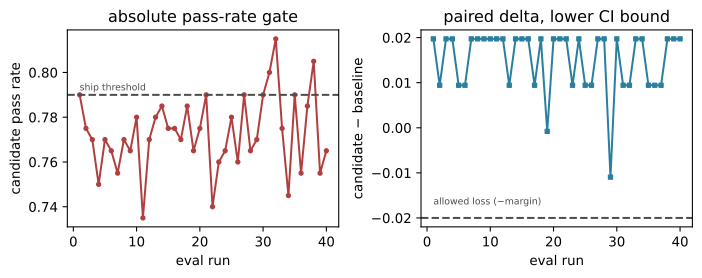
The gate. Given a trustworthy judge, the second decision is the statistic. The naive gate is an absolute bar: ship if the candidate’s pass rate clears a threshold. It flakes, because judge nondeterminism and a small evaluation set make the observed rate wobble run to run, so the same pull request gets a different verdict depending on which night you looked. The senior gate is paired: compute a per-item candidate-minus-baseline delta and put a confidence interval on it, blocking only if the lower bound drops below an allowed loss — the release rule Chapter 22 owns (Section 22.7). It is stable for a physical reason worth stating aloud: the same judge grades both systems on the same items, so its errors are correlated across the pair and largely cancel in the delta even as they move each absolute rate. We simulate one candidate that is a true five-point improvement, graded across forty nightly runs.

rng2 = np.random.default_rng(7)
n_items, runs = 200, 40
p_base, p_cand = 0.78, 0.83           # candidate is a genuine 5-point improvement
judge_err = 0.07                       # the judge mislabels this fraction of ambiguous items
threshold, margin, z = 0.79, 0.02, 1.96

difficulty = rng2.random(n_items)      # per-item latent difficulty, shared by both systems
base_true = difficulty < p_base
cand_true = difficulty < p_cand
abs_rate, paired_low = [], []
for _ in range(runs):
    # one judge, re-run nightly: within a run its errors fall on the same ambiguous
    # items (so a paired comparison cancels them), but a fresh draw each run makes
    # the absolute rate wobble around the threshold.
    mask = rng2.random(n_items) < judge_err
    base_g = np.where(mask, ~base_true, base_true)
    cand_g = np.where(mask, ~cand_true, cand_true)
    abs_rate.append(cand_g.mean())
    delta = cand_g.astype(float) - base_g.astype(float)
    se = delta.std(ddof=1) / np.sqrt(n_items)
    paired_low.append(delta.mean() - z * se)

abs_rate, paired_low = np.array(abs_rate), np.array(paired_low)
ship_abs = int((abs_rate >= threshold).sum())
ship_pair = int((paired_low > -margin).sum())
print(f"absolute gate (ship if rate >= {threshold:.2f}): SHIP {ship_abs}/{runs}, BLOCK {runs - ship_abs}/{runs}  -> flaky")
print(f"paired gate  (ship if CI low > -{margin:.2f}) : SHIP {ship_pair}/{runs}                 -> stable")

fig, axes = plt.subplots(1, 2, figsize=(7.4, 3.0), sharex=True)
xs = range(1, runs + 1)
axes[0].plot(xs, abs_rate, marker="o", ms=3, color="#b13f3f")
axes[0].axhline(threshold, ls="--", color="0.3")
axes[0].text(1, threshold + 0.002, "ship threshold", fontsize=7, color="0.3")
axes[0].set(title="absolute pass-rate gate", xlabel="eval run", ylabel="candidate pass rate")
axes[1].plot(xs, paired_low, marker="s", ms=3, color="#2a7f9e")
axes[1].axhline(-margin, ls="--", color="0.3")
axes[1].text(1, -margin + 0.003, "allowed loss (−margin)", fontsize=7, color="0.3")
axes[1].set(title="paired delta, lower CI bound", xlabel="eval run", ylabel="candidate − baseline")
fig.tight_layout()
plt.show()

absolute gate (ship if rate >= 0.79): SHIP 8/40, BLOCK 32/40  -> flaky
paired gate  (ship if CI low > -0.02) : SHIP 40/40                 -> stable

Figure 37.3: Why does an absolute threshold flake while a paired interval holds? Left: the candidate’s absolute pass rate crosses the ship line run to run. Right: the paired delta’s lower confidence bound stays above the allowed loss on every run — the correlated judge error cancels in the pairing.

The same change, same data, same judge: the absolute gate ships it on some nights and blocks it on others, while the paired gate ships it every time, as Figure 37.3 makes visible. When the interviewer pushes further — “what if the interval is wider than the effect you care about?” — the honest answer is to grow the dataset or buy a repeated-run budget until the interval tightens, never to lower the bar to make a flaky gate pass. Widening the confidence interval is a request for more evidence, not a reason to decide on less.

37.5 Deep dive: the release funnel and its cost tiers

A change does not go from merge to fleet in one hop; it descends a funnel where each tier trades detection speed for coverage and cost, shown in Figure 37.4. The design principle is that the blocking tier must be fast and small while the thorough tiers run out of band — which is exactly what the cost arithmetic in move 2 buys us permission to do.

flowchart LR
    PR["pull request"] --> CI["pinned golden CI gate<br/>&lt; 5 min · paired · blocking"]
    CI -->|block| DEV["back to author"]
    CI -->|pass| RE["replay logged traffic<br/>nightly · Batch API"]
    RE --> CAN["canary 5–10%<br/>judge-scored vs control"]
    CAN --> AB["A/B<br/>outcome metrics"]
    AB --> SHIP["ship to fleet"]
    CAN -. "per-slice regress" .-> ROLL["auto-rollback"]

Figure 37.4: How does a change reach the fleet without a quality regression, and where does each tier’s cost land? The blocking gate is small and fast; the thorough tiers run out of band, on Batch, and on live traffic.

The blocking CI gate grades a small pinned golden set with the paired rule; it clears five minutes because it grades hundreds of items, not thousands. The nightly replay runs the full suite over logged traffic on the Batch API — the tier that is cheap precisely because it tolerates a same-day answer. The canary scores five to ten percent of real traffic with the async judge against a control, and it is the first tier that can catch what offline replay cannot: a drift the frozen eval set never anticipated (the online-eval mechanics are Chapter 27’s, Section 27.5). The A/B tier finally reads outcome metrics rather than the judge’s proxy. When the interviewer pushes on cost — “forty teams, what stops the eval bill from exploding?” — the answer is the tiering itself: the expensive judge is confined to the small blocking set and to sampled traffic, the full suite rides Batch, and the genuinely scarce resource, human labels, is spent only on calibration, never on routine grading. The one thing that must never move to a cheaper tier is judge calibration, because every other number in the funnel inherits its trustworthiness.

37.6 Tradeoffs, failure, and eval as an attack surface

Every choice above buys something and risks something; Table 37.2 is the table a senior draws unprompted in move 6.

Table 37.2: Choice, cost, what it buys, its risk, and the control that contains it.

Choice	Cost	Buys	Risk	Control
Small pinned golden set in CI	misses subtle drift	a blocking gate under 5 min	the golden set goes stale	mine prod failures into it continuously
Nightly full suite on Batch	same-day, not instant, detection	cheap thorough coverage (~50% off)	latency to detection	accept it, for the non-blocking tier only
LLM-as-judge	bias, drift, self-preference	scales open-ended grading	silent mis-gating	{\kappa \ge 0.60}, cross-family judge, pinned version
Paired delta + CI gate	more compute than a threshold	stable verdicts on small n	interval wider than the effect	grow the dataset or buy repeated runs

The failure modes follow the same rows: the golden set silently ages until it blesses a model that regresses on behaviors it no longer covers (control: the flywheel never stops); the judge drifts after an unpinned model upgrade and every downstream number quietly loses meaning (control: recalibrate on any judge change, and pin the version into the verdict). And the two failures a senior treats as attacks, not accidents. Eval-set contamination: cases mined from production leak into a team’s training data, so the model memorizes the test and the gate waves through a change that learned nothing — the control is a held-out, overlap-checked slice and rotating golden cases, and the platform’s own escaped-regression rate is the alarm that it is happening. Gaming the gate: a team optimizes whatever proxy the judge rewards until the metric climbs and the product does not, the Goodhart failure — the control is a cross-family judge, rotated cases, and reading outcome metrics at the A/B tier so the proxy cannot be the final word. Two more the interviewer expects named: fairness, because a gate that reads only the aggregate will bless a model that is fair on average and unfair per slice, so the gate must enforce per-slice floors and a disparate-failure-burden check, both owned by Chapter 22 (Section 22.6); and cost as an attack surface, because an adversarial or careless team could submit enormous candidates and blow the shared eval budget, so per-team budgets and a per-run dataset cap are controls, not niceties. What pages a human: an escaped regression found in production, and a judge whose kappa falls below the bar — both mean the instrument, not just a candidate, is broken.

37.7 Evolution: build order and a changed requirement

Build order is an evidence-gathering sequence. Ship the pinned golden set and the paired gate for a single team first, and measure the gate’s flake rate and escaped-regression rate before anything else, because those two numbers cap trust in the whole platform. Add the judge-calibration loop with human labels once the gate is stable; add the nightly Batch replay when the golden set alone starts missing drift; add online sampling and the canary when production surprises the offline suite; and only then generalize the dataset and judge registries to all forty teams. Plain top-tier grading and one team before any of the multi-tenant machinery — the same discipline Chapter 33 teaches for retrieval.

Then the interviewer flips one requirement: “quality is not enough — the gate must now block any release that regresses on safety, not just quality.” The senior answer is the delta, not a redraw. The dataset-curation loop gains an adversarial red-team slice of golden must-not-regress cases (Chapter 24 owns the trajectories, Chapter 24). The gate gains a second rule that is not a paired confidence interval — a safety regression is a hard zero-tolerance floor, because unsafe behavior is not something you average away with a good aggregate. The judge-calibration loop adds a safety-classifier calibration alongside the quality judge. Everything else — the two-loop shape, the funnel, the cost tiers, five of the six anchor numbers — does not move. That the same skeleton absorbs a safety mandate by adding a slice and a floor, rather than a new architecture, is the point of the family.

37.8 Interviewer probes

Q. Your candidate beats the baseline on aggregate pass rate and the judge agrees with humans 91 percent of the time. Would you ship? Not on those two numbers. Ninety-one percent agreement is base-rate inflated — I would report kappa, and if the set is skewed the kappa can be near zero. Then I would read the paired lower bound (a positive mean can hide a lower bound below the allowed loss), the per-slice floors (the aggregate can bless a slice that collapsed), and the golden regressions. The aggregate is the least informative number in the packet.

Q. A team says your gate is too flaky — it blocks good pull requests half the time. What do you change? First diagnose which half. If the judge’s position-flip rate is high or its kappa has slipped, the instrument is the problem: recalibrate and pin it. If the judge is sound, the statistic is the problem: I am almost certainly gating on an absolute threshold on a small set, and I move to the paired delta with a confidence interval, then grow the golden set or add a repeated-run budget until the interval is tighter than the effect I care about. What I do not do is lower the bar to make the flakiness disappear.

Q. How do you stop teams from gaming the eval to pass the gate? Assume they will — that is Goodhart, not malice. I grade with a cross-family judge so a team cannot optimize the judge’s own idiosyncrasies, rotate golden cases so a static target cannot be memorized, hold out a contamination-checked slice, and read outcome metrics at the A/B tier where the proxy stops being the final word. And I watch the platform’s escaped-regression rate: a gate that is being gamed passes changes that then regress in production, and that number is where it shows.

37.9 The measurement-infra family

The eval platform is one instance of a family whose product is always a number someone will trust, and every sibling shares the same bones: a calibrated instrument, a versioned dataset, a decision on an honest statistic, and an evidence record. What changes is the fork, and the fork flips which statistic and where the enforcement point sits. Table 37.3 transfers the design to three siblings.

Table 37.3: The measurement-infra family: one number each, one fork each, and the design decision the fork flips.

Sibling design	The number it produces	The fork / changed constraint	What flips in the design
Eval / quality gate (this chapter)	is the candidate better?	who owns ground truth?	per-team versioned datasets and judges; paired-CI gate, out of the hot path
Guardrail / safety classifier (Chapter 24)	is this action safe to allow?	in the request path, hard floor	in-line low-latency classifier; zero-tolerance block, not a CI; policy at the effect point
Observability + audit (Chapter 27)	why did this run, and who authorized it?	trace ≠ audit; sampled vs complete	sampled traces for diagnosis; an unsampled, append-only audit for effects
A/B experimentation (Chapter 28)	did the change move the outcome?	live users, a business metric	randomized assignment; sequential testing; outcome metrics, not a judge proxy

The transfer is mechanical once the shared bones are visible. The guardrail sibling is an eval gate moved into the request path, which is why its instrument must be fast and its decision a hard floor rather than a paired interval — you do not average safety. The audit sibling swaps the judged number for a recorded one and splits the evidence plane in two, because the question “why did this run” (sampled, diagnostic) and “who authorized this effect” (complete, tamper-evident) have opposite retention and mutability needs, the trace-versus-audit split Chapter 27 draws (Section 27.2). The A/B sibling moves the whole thing online and replaces the judge’s proxy with a real outcome, which is why its hard part is randomization and sequential statistics rather than judge calibration. Same skeleton, four numbers, four forks.

37.10 Summary

The measurement-infra interview is won on trust, not coverage. Scoping turned on one fork — who owns ground truth — which made datasets and judges per-team versioned artifacts and the platform the owner of machinery, not the bar. The anchor numbers exposed the family’s trap (gate on Cohen’s kappa, not raw agreement) and its center of gravity (human labels, not compute, are scarce). The two-loop skeleton keeps dataset curation and judge calibration separate; the deep dives gated on a calibrated judge and a paired confidence interval instead of a flaky absolute threshold; and the funnel tiered detection against cost. The family skeleton then carried the same bones to guardrail, audit, and A/B siblings by changing one fork each.

37.11 Exercises

1. Re-run the fork. Suppose the interviewer says ground truth is owned centrally — one org-wide definition of quality. Which rows of Table 37.1 change, does the two-loop skeleton survive, and what is the new failure mode you would name aloud?
2. Push the cost model. Using cost_per_query and the study’s illustrative prices: (a) find the judge input/output token shape at which one grade first exceeds one cent; (b) at what number of daily merges does blocking-CI compute overtake the nightly Batch suite; (c) if human calibration must stay under the day’s compute, how many SME-hours per day does that allow at the stated rate?
3. Break the gate on purpose. In the paired-gate cell, raise judge_err to 0.20 and shrink n_items to 50. Report what happens to the paired lower bound’s stability, then find the smallest n_items that restores a consistent SHIP verdict, and state which real-world lever that corresponds to.
4. The judge that passes kappa but fails anyway. Construct a human/judge label pair (as in the first cell) where global kappa clears 0.60 but failure-recall is under 0.5. Explain in one sentence why the release rule reads both numbers, and which class of production incident the low failure-recall would let through.
5. A different sibling. Work the guardrail/safety-classifier row of Table 37.3 as its own two-minute scope: name its fork, the one anchor number you would compute first, why its gate is a hard floor rather than a paired interval, and where its enforcement point sits relative to the model call (recall Chapter 24).
6. Contamination as an attack. Design the held-out slice and overlap check that would catch eval-set contamination for a team that mines production failures into both its eval set and its fine-tuning data. What overlap statistic would you compute, what threshold would block, and how would the platform’s escaped-regression rate confirm the leak after the fact?
7. Absorb a harder flip (multi-part). The interviewer flips two requirements at once: quality must now be measured online per user rather than only pre-merge, and a data-residency rule forbids sending some teams’ traffic to the shared judge. (a) Redraw only the boxes of Figure 37.2 that change. (b) State which anchor numbers move and which survive. (c) Name the one new failure mode residency introduces and its control.