# @save
from __future__ import annotations

import importlib.util
import math
import sys
import time
import warnings
from dataclasses import dataclass
from pathlib import Path

import torch

warnings.filterwarnings("ignore", message="CUDA initialization")  # CPU-only chapter
GIB = 1024**3


@dataclass(frozen=True)
class TrainingConfig:
    """The shape of a dense decoder-only Transformer training run.

    These eight numbers determine everything this chapter computes:
    parameter count follows from the widths and depths, activation memory
    from the sequence length and width, and communication volume from how
    the resulting tensors are cut across devices. ``n_kv_heads`` matters
    because grouped-query attention (Chapter 3) shrinks the K/V
    projections and therefore the parameter count.

    Args:
        name: A label for printed tables.
        d_model: Residual-stream width, the ``h`` in every memory formula.
        n_layers: Transformer block count.
        n_heads: Query heads per layer.
        n_kv_heads: Key/value heads per layer (equal to ``n_heads`` for
            classic multi-head attention, smaller under GQA).
        d_ff: Feed-forward hidden width (SwiGLU uses three ``d_model x
            d_ff`` matrices).
        vocab_size: Token vocabulary, counted twice for untied input and
            output embeddings.
        seq_len: Training sequence length in tokens.
    """

    name: str
    d_model: int
    n_layers: int
    n_heads: int
    n_kv_heads: int
    d_ff: int
    vocab_size: int
    seq_len: int


LLAMA_7B = TrainingConfig("7B-class", 4096, 32, 32, 32, 11008, 32000, 4096)
LLAMA_70B = TrainingConfig("70B-class", 8192, 80, 64, 8, 28672, 128256, 4096)6 Distributed and Frontier Training
A training run can pass its capacity review and still fail on step one. The weights fit across the accelerators, so the plan looks safe — then Adam allocates its moment buffers and the first rank dies out of memory. A second plan survives initialization but spends a third of every step waiting on a pipeline that is mostly bubble. A third loses forty minutes of work to every hardware failure because checkpoints were an afterthought. Each failure is the same mistake: treating distributed training as “put the model on more GPUs” instead of as arithmetic that must balance several ledgers — bytes, seconds, and dollars — at once.
We are now ready to build that arithmetic as code we can run: (i) a memory calculator that prices every byte of a training step for a real seven-billion-parameter configuration, under full precision, mixed precision, and each ZeRO sharding stage; (ii) an activation model checked against a live measurement of what autograd actually saves; (iii) a simulator for tensor, pipeline, and data parallelism that takes a cluster and a model and returns per-device memory, pipeline bubble, and communication volume for every legal layout; (iv) a model-FLOPs-utilization number computed honestly from a matmul benchmark and a measured training loop; (v) a checkpoint-interval optimizer with a worked answer; and (vi) a cost model that turns Chapter 5’s compute budget into device-hours, dollars, and megawatts for three named-scale runs. None of this needs a cluster. That is the point: the planning arithmetic that decides how frontier runs are laid out is exactly the arithmetic on these pages, and all of it runs on a laptop.
6.1 The memory ledger of one training step
Everything in this chapter prices some resource against a model configuration, so we start by writing the configuration down. The fields are the ones that determine parameter count and activation size; the two instances are the shapes of two widely trained open models, which lets us check our arithmetic against published numbers instead of against our own assumptions.
From shapes to parameters is bookkeeping we already did once for a toy model in Chapter 2; here we redo it with grouped-query attention so that the calculator reproduces real checkpoints, not just round numbers.
# @save
def param_count(cfg: TrainingConfig) -> dict[str, int]:
    """Count parameters per component from the configuration's shapes.

    Attention costs one ``d x d`` matrix each for the query and output
    projections plus two ``d x (d_head * n_kv_heads)`` matrices for keys
    and values; a SwiGLU feed-forward block costs three ``d x d_ff``
    matrices; untied embeddings appear once at the input and once at the
    LM head. Norm scales and biases are omitted — they are parts in ten
    thousand at these widths.

    Args:
        cfg: The model configuration to price.

    Returns:
        Parameter counts for ``"attention"``, ``"ffn"``, and
        ``"embeddings"``, plus a ``"total"`` entry summing them.
    """
    d = cfg.d_model
    kv_width = (d // cfg.n_heads) * cfg.n_kv_heads
    attention = cfg.n_layers * (2 * d * d + 2 * d * kv_width)
    ffn = cfg.n_layers * 3 * d * cfg.d_ff
    embeddings = 2 * cfg.vocab_size * d
    total = attention + ffn + embeddings
    return {"attention": attention, "ffn": ffn, "embeddings": embeddings, "total": total}
Does the bookkeeping survive contact with reality? Run it on both configurations:
for cfg in (LLAMA_7B, LLAMA_70B):
    counts = param_count(cfg)
    parts = {name: f"{value / 1e9:.2f}B" for name, value in counts.items()}
    print(f"{cfg.name:9s} {parts}")
7B-class {'attention': '2.15B', 'ffn': '4.33B', 'embeddings': '0.26B', 'total': '6.74B'}
70B-class {'attention': '12.08B', 'ffn': '56.37B', 'embeddings': '2.10B', 'total': '70.55B'}Both totals land on the published sizes — 6.74B and 70.6B — from shapes alone, which is our license to trust the rest of the ledger. Now the question that decides whether a run fits: how many bytes does training attach to each of those parameters?
Storing a weight is the cheap part. A training step must also hold a gradient for every weight, and Adam — still the default optimizer at scale — keeps two exponential moving averages (the first and second moments) per weight, in fp32. Mixed-precision training adds one more tenant: the forward and backward passes run on bf16 copies of the weights, while an fp32 master copy accumulates the updates so that tiny increments do not round away. Per parameter, the standard recipe is
M_{\text{state}} = \underbrace{2}_{\text{bf16 weight}} + \underbrace{2}_{\text{bf16 gradient}} + \underbrace{4}_{\text{fp32 master}} + \underbrace{8}_{\text{fp32 moments}} = 16 \ \text{bytes}, \tag{6.1}
so a model of P parameters carries {16}P bytes of persistent optimizer-visible state before a single activation exists. We encode the recipe as data so we can swap it later, and the ledger as a function so we can shard it later.
# @save
PRECISION_RECIPES = {
    "fp32": {"weights": 4, "gradients": 4, "master weights": 0, "Adam moments": 8},
    "mixed": {"weights": 2, "gradients": 2, "master weights": 4, "Adam moments": 8},
}


def state_ledger(
    params: int, recipe: str = "mixed", zero_stage: int = 0, shards: int = 1
) -> dict[str, float]:
    """Price the persistent training state a single device must hold.

    The ledger multiplies the parameter count by bytes-per-parameter for
    each state component, then divides the components that the chosen
    ZeRO stage shards across ``shards`` data-parallel devices: stage 1
    shards the fp32 master weights and Adam moments, stage 2 also shards
    gradients, stage 3 also shards the bf16 weights themselves (gathering
    them transiently per block during compute). Activations are priced
    separately — they live on a different schedule.

    Args:
        params: Trainable parameter count.
        recipe: Key into ``PRECISION_RECIPES`` (``"fp32"`` or ``"mixed"``).
        zero_stage: 0 (fully replicated) through 3 (fully sharded).
        shards: Devices in the sharding group.

    Returns:
        Bytes per device for each component plus a ``"total"`` entry.
    """
    sharded_from = {"master weights": 1, "Adam moments": 1, "gradients": 2, "weights": 3}
    ledger = {
        component: params * bytes_per / (shards if zero_stage >= sharded_from[component] else 1)
        for component, bytes_per in PRECISION_RECIPES[recipe].items()
    }
    ledger["total"] = sum(ledger.values())
    return ledger
Run it for the 7B configuration under both precision recipes and watch for the surprise:
P_7B = param_count(LLAMA_7B)["total"]
for recipe in ("fp32", "mixed"):
    ledger = state_ledger(P_7B, recipe)
    row = {name: f"{value / GIB:6.1f}" for name, value in ledger.items()}
    print(f"{recipe:5s} GiB: {row}")
fp32 GiB: {'weights': ' 25.1', 'gradients': ' 25.1', 'master weights': ' 0.0', 'Adam moments': ' 50.2', 'total': ' 100.4'}
mixed GiB: {'weights': ' 12.6', 'gradients': ' 12.6', 'master weights': ' 25.1', 'Adam moments': ' 50.2', 'total': ' 100.4'}Both recipes total 100.4 GiB. Mixed precision does not shrink training state at all — the bf16 savings on weights and gradients are exactly cancelled by the fp32 master copy it adds. What mixed precision buys is elsewhere: activations at half the bytes, matmuls on tensor cores at several times the throughput, and half the gradient bytes on the wire. The 12 fp32 bytes of optimizer state per parameter survive untouched, which is why the optimizer, not the model, is the first thing sharding attacks in Section 6.3. FP8 recipes push the same idea further — narrower tensors with per-block scaling factors, higher-precision islands for softmax and reductions (DeepSeek-AI et al. 2024) — and change the recipe dict, not the ledger logic; the current formats live in this chapter’s dated landscape box.
The headline: a 6.74B-parameter model needs 100.4 GiB of state, and a typical training accelerator has 80 GiB. The model that “fits” — 12.6 GiB of bf16 weights would fit six times over — cannot train on one device. And we have not yet counted the largest and most misunderstood tenant of all.
6.2 Activations, and buying memory with FLOPs
Backward passes reuse forward results: to differentiate a matmul, autograd needs the input it saw during the forward pass, so every intermediate tensor the forward pass produces is a candidate for being saved until the backward pass consumes it. Those saved tensors are the activation memory, and unlike optimizer state they scale with batch size and sequence length rather than with parameter count. For one Transformer layer processing b sequences of s tokens at width h with a attention heads, a careful census of the saved tensors (Korthikanti et al. 2022) gives, in bf16,
A_{\text{layer}} \approx 34\,s\,b\,h \;+\; 5\,a\,s^{2}\,b \ \text{bytes}. \tag{6.2}
The first term collects the linear-layer inputs, norms, and activation functions — every tensor of shape s \times b \times h the layer touches, and there are about seventeen of them at two bytes each. The second term is the attention matrix itself: scores and softmax weights of shape a \times s \times s per sequence, the quadratic culprit from Chapter 3. A fused attention kernel such as FlashAttention (Dao et al. 2022) never materializes that matrix — it recomputes score tiles on the fly during backward — which deletes the second term entirely. Full activation checkpointing goes further: save only each block’s input ({2}\,s\,b\,h bytes), throw everything else away, and recompute the block’s forward pass from that input when backward needs it. Three policies, one function:
# @save
def activation_bytes_per_layer(cfg: TrainingConfig, microbatch: int, policy: str) -> float:
    """Price the tensors autograd saves per layer under a memory policy.

    ``"materialize scores"`` is naive attention: every linear input plus
    the ``a x s x s`` score and softmax tensors. ``"fused attention"``
    keeps the linear inputs but never stores the score matrix (the
    FlashAttention effect). ``"full recompute"`` checkpoints the block:
    only its input survives the forward pass, and the rest is recomputed
    during backward at the cost of roughly one extra forward pass.

    Args:
        cfg: The model configuration (supplies ``s``, ``h``, and ``a``).
        microbatch: Sequences per device per forward pass (the ``b``).
        policy: One of the three policy names above.

    Returns:
        Saved bytes per layer, assuming two-byte activations.

    Raises:
        ValueError: If ``policy`` is not one of the three names.
    """
    s, b, h = cfg.seq_len, microbatch, cfg.d_model
    if policy == "materialize scores":
        return 34 * s * b * h + 5 * cfg.n_heads * s * s * b
    if policy == "fused attention":
        return 34 * s * b * h
    if policy == "full recompute":
        return 2 * s * b * h
    raise ValueError(f"unknown activation policy: {policy}")
Price the 7B configuration under each policy, one 4,096-token sequence per device:
for policy in ("materialize scores", "fused attention", "full recompute"):
    per_layer = activation_bytes_per_layer(LLAMA_7B, 1, policy)
    total = per_layer * LLAMA_7B.n_layers
    print(f"{policy:19s} {per_layer / GIB:6.3f} GiB/layer   {total / GIB:5.1f} GiB for 32 layers")
materialize scores 3.031 GiB/layer 97.0 GiB for 32 layers
fused attention 0.531 GiB/layer 17.0 GiB for 32 layers
full recompute 0.031 GiB/layer 1.0 GiB for 32 layersRead the totals against the 100.4 GiB of state. Naive attention would add 97 GiB of activations for a single sequence per device — at sequence length 4,096, the score matrices alone rival the optimizer. The fused kernel cuts that to 17 GiB, and full recomputation to about 1 GiB, at the price of roughly one extra forward pass — about a third more compute per step, since backward costs about twice forward. That trade, FLOPs for bytes, is the first knob every large run turns.
A formula this load-bearing should be checked against reality at least once. We reuse the TinyGPT we trained in Chapter 2, and count the saved bytes directly: torch.autograd.graph.saved_tensors_hooks lets us intercept every tensor autograd stashes for backward, so we can measure the true activation footprint of a forward/backward pass — first plain, then with torch.utils.checkpoint wrapping each block.
# @save
def load_chapter_module(chapter: str, name: str):
    """Import an earlier chapter's tangled teaching module by path.

    Each finished chapter tangles its ``# @save`` cells into
    ``code/chNN/_generated.py``. This helper walks up from the working
    directory to the book root and imports the requested module under a
    fresh name, so later chapters build on earlier artifacts instead of
    re-implementing them.

    Args:
        chapter: Chapter code directory, e.g. ``"ch02"``.
        name: Module name to register, e.g. ``"ch02_generated"``.

    Returns:
        The executed module object.
    """
    root = Path.cwd()
    while not (root / "code" / chapter / "_generated.py").exists():
        if root.parent == root:
            raise FileNotFoundError(f"cannot find code/{chapter}/_generated.py")
        root = root.parent
    spec = importlib.util.spec_from_file_location(name, root / "code" / chapter / "_generated.py")
    module = importlib.util.module_from_spec(spec)
    sys.modules[name] = module
    spec.loader.exec_module(module)
    return module
With the loader in hand, we instantiate a slightly-scaled-up TinyGPT — four layers, width 128 — as our measurement subject:
ch02 = load_chapter_module("ch02", "ch02_generated")
tiny_config = ch02.GPTConfig(vocab_size=256, block_size=128, d_model=128, n_heads=4, n_layers=4, mlp_ratio=4)
torch.manual_seed(6)
tiny = ch02.TinyGPT(tiny_config)
print(f"TinyGPT for the measurement: {sum(p.numel() for p in tiny.parameters()):,} parameters")
TinyGPT for the measurement: 1,099,136 parametersThe measurement itself runs the model’s blocks by hand so we can flip checkpointing on and off, with a hook that adds up bytes as autograd saves tensors:
# @save
def measure_saved_bytes(model, tokens: torch.Tensor, targets: torch.Tensor, checkpoint_blocks: bool) -> int:
    """Measure the bytes autograd saves during one forward/backward pass.

    Registers a ``saved_tensors_hooks`` pair that counts every tensor the
    autograd graph stores for backward, then runs the model's blocks
    either plainly or wrapped in ``torch.utils.checkpoint`` (which saves
    only each block's input and recomputes the interior during backward).
    The count is ground truth for the policy comparison that
    ``activation_bytes_per_layer`` only models.

    Args:
        model: A Chapter 2 ``TinyGPT`` whose blocks we drive manually.
        tokens: Input token ids of shape ``(batch, seq)``.
        targets: Next-token targets of the same shape.
        checkpoint_blocks: Whether to checkpoint each block.

    Returns:
        Total bytes of tensors saved for the backward pass.
    """
    from torch.utils.checkpoint import checkpoint as run_checkpointed

    saved = 0

    def record(tensor: torch.Tensor) -> torch.Tensor:
        nonlocal saved
        saved += tensor.numel() * tensor.element_size()
        return tensor

    positions = torch.arange(tokens.size(1))
    with torch.autograd.graph.saved_tensors_hooks(record, lambda tensor: tensor):
        x = model.token_embedding(tokens) + model.position_embedding(positions)
        for block in model.blocks:
            step = lambda value, layer=block: layer(value)[0]
            x = run_checkpointed(step, x, use_reentrant=False) if checkpoint_blocks else step(x)
        logits = model.lm_head(model.final_norm(x))
        loss = torch.nn.functional.cross_entropy(logits.flatten(0, 1), targets.flatten())
        loss.backward()
    return saved
Run it both ways on the same batch and compare what autograd actually kept:
torch.manual_seed(6)
tokens = torch.randint(tiny_config.vocab_size, (4, tiny_config.block_size))
targets = torch.roll(tokens, -1, dims=1)
plain = measure_saved_bytes(tiny, tokens, targets, checkpoint_blocks=False)
tiny.zero_grad(set_to_none=True)
checkpointed = measure_saved_bytes(tiny, tokens, targets, checkpoint_blocks=True)
print(f"saved tensors, plain       : {plain:>12,} bytes")
print(f"saved tensors, checkpointed: {checkpointed:>12,} bytes  ({1 - checkpointed / plain:.1%} less)")
saved tensors, plain : 50,711,044 bytes
saved tensors, checkpointed: 3,290,628 bytes (93.5% less)A 94% reduction — measured, not modeled. The exact ratio is configuration-dependent: this toy materializes its attention score matrices (no fused kernel here) and stores fp32 activations, so its ledger has different constants than Equation 6.2’s — exactly the kind of drift a formula hides and a hook exposes. The shape of the result, though, is the one the model predicts: checkpointing leaves almost nothing beyond the block boundaries. Recomputation must also be semantically identical — dropout needs the same RNG state on replay — which frameworks handle but custom blocks can break; one matched-loss check from identical weights is cheap insurance. Figure 6.1 puts the model’s three policies next to the state ledger they compete with.
Show the code that draws this figure
import matplotlib.pyplot as plt

policies = ["materialize scores", "fused attention", "full recompute"]
totals = [
    activation_bytes_per_layer(LLAMA_7B, 1, policy) * LLAMA_7B.n_layers / GIB
    for policy in policies
]
fig, ax = plt.subplots(figsize=(6.2, 3.2))
bars = ax.bar(policies, totals, color=["0.75", "0.55", "0.35"], width=0.55)
ax.bar_label(bars, fmt="%.1f GiB", padding=2, fontsize=9)
state_gib = state_ledger(P_7B)["total"] / GIB
ax.axhline(state_gib, ls=":", color="0.3")
ax.text(2.42, state_gib * 1.12, "training state 100.4 GiB", ha="right", fontsize=8)
ax.axhline(80, ls="--", color="0.6")
ax.text(2.42, 60, "one 80 GiB device", ha="right", fontsize=8, color="0.35")
ax.set_yscale("log")
ax.set_ylabel("activation GiB (log scale)")
ax.set_ylim(0.5, 300)
fig.tight_layout()
plt.show()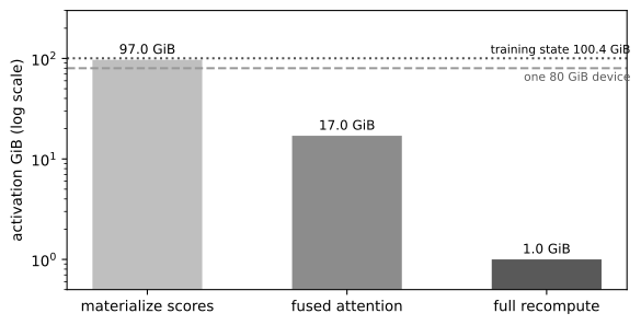
6.3 Sharding the state: ZeRO and FSDP
Data parallelism is the oldest scaling move: give every device a full replica of the model, feed each a different slice of the batch, and all-reduce the gradients so every replica applies the same update. It multiplies throughput, and it multiplies nothing else — each of n replicas still holds all {16}P bytes. The observation behind ZeRO (Rajbhandari et al. 2020) is that this replication is almost entirely waste: the optimizer states, gradients, and even the weights are identical across replicas, so each replica could own just {1/n}-th of them and borrow the rest when needed. Each ZeRO stage removes one class of replication, and our state_ledger already knows how, via its zero_stage argument:
for stage in range(4):
    total = state_ledger(P_7B, "mixed", zero_stage=stage, shards=8)["total"]
    label = ("replicated (DDP)", "ZeRO-1", "ZeRO-2", "ZeRO-3 / FSDP")[stage]
    print(f"stage {stage} {label:17s} {total / GIB:6.1f} GiB per device over 8")
stage 0 replicated (DDP) 100.4 GiB per device over 8
stage 1 ZeRO-1 34.5 GiB per device over 8
stage 2 ZeRO-2 23.5 GiB per device over 8
stage 3 ZeRO-3 / FSDP 12.6 GiB per device over 8Stage 1 shards the fp32 master weights and moments — the 12-byte tenant from Equation 6.1 — and per-device state collapses from 100.4 to 34.5 GiB: the single cheapest memory win in distributed training, because the optimizer only ever touches its own shard (each device updates its own slice of the parameters, then the updated slices are gathered). Stage 2 also shards gradients, which costs nothing extra in communication: the all-reduce every replica already performed is reorganized as a reduce-scatter (each device keeps only its shard of the summed gradient) followed by an all-gather of updated weights — the same bytes on the wire, differently bracketed. Stage 3 — the design PyTorch ships as FSDP (Zhao et al. 2023) — shards the weights themselves. Now a device does not even hold the full bf16 model; before computing a block it all-gathers that block’s weight shards from the group, uses them, and frees them. The per-device floor drops to {16}P/n, and the price is a third parameter-sized collective per step: relative to DDP’s two gradient volumes, ZeRO-3 moves roughly three (weights gathered for forward, gathered again for backward, gradients reduce-scattered).
Figure 6.2 shows the whole progression by component, and the sequence in Figure 6.3 shows when the bytes exist — the part totals hide.
Show the code that draws this figure
plans = [
    ("fp32\nDDP", state_ledger(P_7B, "fp32")),
    ("mixed\nDDP", state_ledger(P_7B, "mixed")),
    ("ZeRO-1\nover 8", state_ledger(P_7B, "mixed", 1, 8)),
    ("ZeRO-2\nover 8", state_ledger(P_7B, "mixed", 2, 8)),
    ("ZeRO-3\nover 8", state_ledger(P_7B, "mixed", 3, 8)),
]
components = ["weights", "gradients", "master weights", "Adam moments"]
shades = ["0.25", "0.45", "0.65", "0.82"]
fig, ax = plt.subplots(figsize=(6.4, 3.4))
bottoms = [0.0] * len(plans)
for component, shade in zip(components, shades):
    heights = [ledger[component] / GIB for _, ledger in plans]
    ax.bar([label for label, _ in plans], heights, bottom=bottoms, color=shade,
           label=component, width=0.6, edgecolor="white", linewidth=0.4)
    bottoms = [base + height for base, height in zip(bottoms, heights)]
for index, (label, ledger) in enumerate(plans):
    ax.text(index, ledger["total"] / GIB + 2, f"{ledger['total'] / GIB:.0f}", ha="center", fontsize=9)
ax.axhline(80, ls="--", color="0.5")
ax.text(4.4, 82, "80 GiB device", ha="right", fontsize=8, color="0.35")
ax.set_ylabel("GiB per device")
ax.legend(frameon=False, fontsize=8, ncol=2)
fig.tight_layout()
plt.show()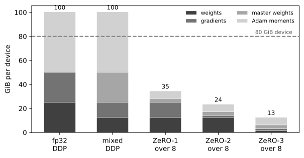
sequenceDiagram
    participant R0 as Rank 0
    participant R1 as Rank 1
    participant A as Autograd
    R0->>R1: all-gather block weight shards
    R1->>R0: all-gather block weight shards
    Note over R0,R1: full block weights exist (transient)
    R0->>R0: forward on local microbatch
    R1->>R1: forward on local microbatch
    R0-->>A: save block input only (checkpointing)
    R1-->>A: save block input only (checkpointing)
    Note over R0,R1: reshard - full weights freed
    A->>R0: backward reaches this block
    A->>R1: backward reaches this block
    R0->>R1: all-gather again, recompute, differentiate
    R1->>R0: all-gather again, recompute, differentiate
    R0->>R1: reduce-scatter gradient shards
    R1->>R0: reduce-scatter gradient shards
Two practical notes complete the picture. First, granularity: FSDP gathers weights one unit at a time — usually one Transformer block — so peak memory includes the persistent shard plus the largest transiently gathered unit, and prefetching the next block’s gather behind the current block’s compute raises the peak again. Second, hybrid sharding (HSDP): sharding over all 128 devices of a cluster puts latency-sensitive all-gathers across slow inter-node links, so real deployments shard within a fast domain (say, 8 devices in a node) and replicate across domains — per-device state is {16}P/8, not {16}P/128, in exchange for keeping the frequent collectives on the fast fabric. Which fabric is fast enough for what is precisely the question the next two sections quantify.
6.4 Splitting the computation: tensor and pipeline parallelism
ZeRO shards storage, but every device still executes every layer. Two situations break that: a layer’s computation is too big for one device to finish in acceptable time, or — at 70B and beyond — even the sharded state plus one gathered block strains memory. Then we split the computation itself, and the two classic cuts slice in orthogonal directions: tensor parallelism splits within each layer, pipeline parallelism splits across layers.
Tensor parallelism (Shoeybi et al. 2019) rests on one matrix identity. Split a feed-forward block’s up-projection by columns across two devices and each device computes half the hidden features — no communication needed, because each output column depends on all of the input, which both devices hold. Then split the down-projection by rows: each device consumes exactly the hidden half it already has, and produces a partial sum of the full output. One all-reduce adds the partials. The nonlinearity between the two matmuls applies elementwise to each half, so it never forces communication. We can verify the identity in a few lines:
# @save
def tensor_parallel_ffn(
    x: torch.Tensor, w_up: torch.Tensor, w_down: torch.Tensor, shards: int
) -> torch.Tensor:
    """Run a two-matmul FFN split column-then-row across simulated shards.

    The up-projection is split by output columns (each shard computes a
    slice of the hidden features from the full input), the down-projection
    by input rows (each shard consumes exactly its own hidden slice and
    emits a partial sum of the output). Summing the partials — the one
    all-reduce a Megatron-style block performs per matmul pair — must
    reproduce the unsharded result up to float round-off.

    Args:
        x: Input activations of shape ``(batch, d_model)``.
        w_up: Up-projection weight of shape ``(d_model, d_ff)``.
        w_down: Down-projection weight of shape ``(d_ff, d_model)``.
        shards: How many tensor-parallel devices to simulate.

    Returns:
        The combined output, mathematically equal to
        ``relu(x @ w_up) @ w_down``.
    """
    up_shards = w_up.chunk(shards, dim=1)
    down_shards = w_down.chunk(shards, dim=0)
    partials = [torch.relu(x @ up) @ down for up, down in zip(up_shards, down_shards)]
    return torch.stack(partials).sum(dim=0)
Check it against the unsharded computation:
torch.manual_seed(0)
x = torch.randn(4, 256)
w_up, w_down = torch.randn(256, 1024) / 16, torch.randn(1024, 256) / 32
reference = torch.relu(x @ w_up) @ w_down
for shards in (2, 4):
    gap = (tensor_parallel_ffn(x, w_up, w_down, shards) - reference).abs().max()
    print(f"{shards}-way tensor parallel vs single device: max |difference| = {gap.item():.2e}")
2-way tensor parallel vs single device: max |difference| = 4.77e-07
4-way tensor parallel vs single device: max |difference| = 5.96e-07The sharded and unsharded results agree to float round-off — the split is exact in exact arithmetic. Attention shards the same way (heads split naturally by columns), so a full Transformer layer costs two all-reduces in forward and two in backward. That frequency is tensor parallelism’s defining constraint: the collectives sit on the critical path of every layer, so the payloads better be on the fastest links you own. How much traffic?
# @save
def tp_comm_bytes_per_layer(cfg: TrainingConfig, microbatch: int, tp: int, scalar_bytes: int = 2) -> float:
    """Estimate per-device tensor-parallel traffic for one layer's fwd+bwd.

    A Megatron-style layer performs four all-reduces per microbatch (two
    forward, two backward), each over the ``s x b x h`` activation tensor.
    A ring all-reduce moves ``2 (tp - 1) / tp`` times the payload per
    participating device. This is a leading-order planning number: it
    ignores latency terms and any sequence-parallel optimizations.

    Args:
        cfg: The model configuration (supplies ``s`` and ``h``).
        microbatch: Sequences per device per forward pass.
        tp: Tensor-parallel degree (1 means no traffic).
        scalar_bytes: Bytes per activation scalar (two for bf16).

    Returns:
        Bytes per device per layer per microbatch.
    """
    if tp == 1:
        return 0.0
    payload = cfg.seq_len * microbatch * cfg.d_model * scalar_bytes
    return 4 * 2 * (tp - 1) / tp * payload
Price an 8-way split of the 7B model:
per_layer = tp_comm_bytes_per_layer(LLAMA_7B, 1, 8)
print(f"tp=8 on the 7B: {per_layer / GIB:.3f} GiB/layer/microbatch, "
      f"{per_layer * LLAMA_7B.n_layers / GIB:.1f} GiB per microbatch across 32 layers")
tp=8 on the 7B: 0.219 GiB/layer/microbatch, 7.0 GiB per microbatch across 32 layersSeven gibibytes of collective traffic per microbatch — per device — explains the standard placement rule: tensor parallelism stays inside a node (NVLink-class links, hundreds of GB/s), and its degree rarely exceeds 8.
Pipeline parallelism cuts the other way: stage 0 gets the first few layers, stage 1 the next few, and only the block-boundary activation crosses between stages — kilobytes-to-megabytes per microbatch instead of gibibytes, which is why pipelines happily span nodes. The catch is time, not traffic. With one batch in flight, stage 1 idles while stage 0 computes and vice versa. The fix is to split the batch into m microbatches and stream them, so stages work on different microbatches simultaneously; the residual idleness — the pipeline bubble — is the fill-and-drain time at the schedule’s ends. For S balanced stages,
f_{\text{bubble}} = \frac{S - 1}{m + S - 1}, \tag{6.3}
the fraction of each device’s time spent waiting (Huang et al. 2019). Rather than trust the formula, we simulate the schedule that production systems actually run — one-forward-one-backward, or 1F1B (Narayanan et al. 2021), which interleaves each microbatch’s backward as early as dependencies allow to bound how many activations a stage holds. First, the order of operations each stage executes:
# @save
def one_f1b_order(stage: int, stages: int, microbatches: int) -> list[tuple[str, int]]:
    """Return the (kind, microbatch) sequence a 1F1B stage executes.

    Each stage runs a warmup of forwards — more for earlier stages, so
    later stages have work queued — then strictly alternates backward and
    forward until forwards run out, and drains the remaining backwards.
    The early backwards are what let a stage free each microbatch's
    activations promptly instead of holding all ``m`` at once.

    Args:
        stage: This stage's index, 0-based from the front.
        stages: Total pipeline stages.
        microbatches: Microbatches per optimizer step.

    Returns:
        Ordered ``("F", m)`` / ``("B", m)`` work items for this stage.
    """
    warmup = min(microbatches, stages - stage)
    ops = [("F", micro) for micro in range(1, warmup + 1)]
    forward_next = warmup + 1
    for backward in range(1, microbatches + 1):
        ops.append(("B", backward))
        if forward_next <= microbatches:
            ops.append(("F", forward_next))
            forward_next += 1
    return ops
Then a small discrete-event simulator: an operation starts when its stage is free and its dependency has finished — a forward needs the previous stage’s forward of the same microbatch, a backward needs the next stage’s backward plus its own forward.
# @save
def simulate_pipeline(
    stages: int, microbatches: int, forward_time: float = 1.0, backward_time: float = 2.0
) -> tuple[list[tuple], float, float]:
    """Simulate a 1F1B pipeline schedule and measure its idle fraction.

    Walks each stage's 1F1B work order under the true dependency rules
    (a forward waits on the upstream forward; a backward waits on the
    downstream backward and the local forward), packing operations
    greedily. The returned idle fraction is measured from the resulting
    timeline, so it can be checked against the closed-form bubble
    formula instead of assumed from it.

    Args:
        stages: Pipeline stages (devices in the pipeline group).
        microbatches: Microbatches per optimizer step.
        forward_time: Time units per microbatch forward on one stage.
        backward_time: Time units per microbatch backward (about twice
            the forward cost for a Transformer block).

    Returns:
        A tuple of the event list ``(stage, kind, microbatch, start,
        duration)``, the makespan, and the measured idle fraction.
    """
    orders = {k: one_f1b_order(k, stages, microbatches) for k in range(stages)}
    finish: dict[tuple[str, int, int], float] = {}
    events, free, pointer = [], [0.0] * stages, [0] * stages
    remaining = sum(len(ops) for ops in orders.values())
    while remaining:
        progressed = False
        for stage in range(stages):
            if pointer[stage] == len(orders[stage]):
                continue
            kind, micro = orders[stage][pointer[stage]]
            if kind == "F":
                needs = ("F", micro, stage - 1) if stage else None
            else:
                needs = ("B", micro, stage + 1) if stage < stages - 1 else ("F", micro, stage)
            if needs is not None and needs not in finish:
                continue
            ready = finish.get(needs, 0.0)
            if kind == "B":
                ready = max(ready, finish[("F", micro, stage)])
            start = max(free[stage], ready)
            duration = forward_time if kind == "F" else backward_time
            finish[(kind, micro, stage)] = start + duration
            events.append((stage, kind, micro, start, duration))
            free[stage] = start + duration
            pointer[stage] += 1
            remaining -= 1
            progressed = True
        if not progressed:
            raise RuntimeError("schedule deadlocked; a dependency can never be met")
    makespan = max(start + duration for *_, start, duration in events)
    busy = microbatches * (forward_time + backward_time)
    return events, makespan, 1.0 - busy / makespan
Now the check — the simulator measures idleness from its own timeline, the formula predicts it:
def pipeline_bubble_fraction(stages: int, microbatches: int) -> float:
    """Closed-form 1F1B fill-and-drain bubble fraction for balanced stages."""
    return (stages - 1) / (microbatches + stages - 1)


for stages, microbatches in ((4, 8), (8, 32), (8, 8)):
    _, _, measured = simulate_pipeline(stages, microbatches)
    predicted = pipeline_bubble_fraction(stages, microbatches)
    print(f"S={stages} m={microbatches:2d}: simulated idle {measured:.4f}   formula {predicted:.4f}")
S=4 m= 8: simulated idle 0.2727 formula 0.2727
S=8 m=32: simulated idle 0.1795 formula 0.1795
S=8 m= 8: simulated idle 0.4667 formula 0.4667They agree to four decimals in every case, including with backward set to twice forward — the bubble is a fraction, so uniform scaling of op times cancels. The numbers also show the lever: at eight stages, eight microbatches leaves devices idle 47% of the time; thirty-two microbatches cuts that to 18%. Figure 6.4 draws the simulated timeline so the fill-and-drain triangles stop being abstract. Interleaved schedules (each device hosting several non-contiguous “virtual stages”) shrink the bubble further without needing a larger batch, at the cost of more boundary traffic — same simulator, finer stages.
Show the code that draws this figure
events, makespan, idle = simulate_pipeline(4, 8)
fig, ax = plt.subplots(figsize=(6.6, 2.9))
for stage, kind, micro, start, duration in events:
    color = "0.82" if kind == "F" else "0.45"
    ax.broken_barh([(start, duration)], (3 - stage - 0.38, 0.76), facecolors=color,
                   edgecolor="white", linewidth=0.5)
    ax.text(start + duration / 2, 3 - stage, str(micro), ha="center", va="center",
            fontsize=7, color="black" if kind == "F" else "white")
ax.set_yticks([3, 2, 1, 0], [f"stage {k}" for k in range(4)])
ax.set_xlabel(f"time units (makespan {makespan:.0f}, idle fraction {idle:.0%})")
ax.set_xlim(0, makespan)
handles = [plt.Rectangle((0, 0), 1, 1, fc="0.82"), plt.Rectangle((0, 0), 1, 1, fc="0.45")]
ax.legend(handles, ["forward", "backward"], frameon=False, fontsize=8, loc="lower right")
fig.tight_layout()
plt.show()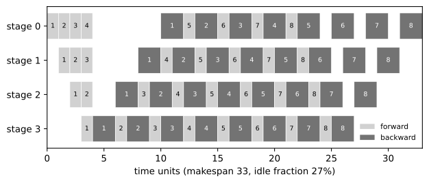
6.5 Composing a plan: the parallelism simulator
We now hold all the parts: state sharding, activation policies, tensor splits, pipeline schedules. A real cluster forces one decision that uses them all — given G devices and a model, choose degrees t \times S \times n = G for tensor, pipeline, and data parallelism. The axes multiply device count, and they compete: every device granted to tensor or pipeline parallelism is a device not granted to data parallelism, and — less spoken — every data-parallel replica takes microbatches away from the pipeline, because a fixed global batch divided over more replicas leaves fewer microbatches per pipeline to amortize the bubble. Composition is where the arithmetic earns its keep, so we make it a function.
# @save
def evaluate_plan(
    cfg: TrainingConfig, tp: int, pp: int, dp: int, *,
    global_batch: int = 128, zero_stage: int = 1, device_gib: float = 80.0,
) -> dict[str, object]:
    """Price one tensor/pipeline/data-parallel layout for a training run.

    Weights are split ``tp * pp`` ways; ZeRO at ``zero_stage`` shards the
    remaining state across the ``dp`` replicas. Activations assume full
    block recomputation (the large-model default): each stage holds one
    boundary tensor per resident layer for up to ``pp`` in-flight
    microbatches, divided by ``tp``, plus one layer's transient
    recompute working set. Communication columns are leading-order bytes
    per device per optimizer step on each axis. Deliberately ignored:
    latency terms, overlap, expert/context axes, and kernel efficiency —
    this is the memory-and-volume sieve that comes before any benchmark.

    Args:
        cfg: The model configuration to lay out.
        tp: Tensor-parallel degree (keep within one node in practice).
        pp: Pipeline-parallel degree.
        dp: Data-parallel degree.
        global_batch: Global batch in sequences; each replica processes
            ``global_batch / dp`` single-sequence microbatches per step.
        zero_stage: ZeRO stage applied across the data-parallel axis.
        device_gib: Device memory used for the feasibility verdict.

    Returns:
        A dict with the plan label, per-device state/activation/total
        GiB, a feasibility flag, bubble percentage, and per-axis
        communication GiB per device per step.
    """
    params_per_shard = param_count(cfg)["total"] / (tp * pp)
    state = state_ledger(params_per_shard, "mixed", zero_stage, dp)
    microbatches = global_batch // dp
    boundary = 2 * cfg.seq_len * cfg.d_model
    layers_here = cfg.n_layers / pp
    inflight = min(pp, microbatches) if pp > 1 else 1
    saved = boundary * layers_here * inflight / tp
    transient = activation_bytes_per_layer(cfg, 1, "fused attention") / tp
    activations = saved + transient
    bubble = (pp - 1) / (microbatches + pp - 1)
    dp_comm = 2 * (dp - 1) / dp * 2 * params_per_shard
    tp_comm = tp_comm_bytes_per_layer(cfg, 1, tp) * layers_here * microbatches
    pp_comm = 2 * boundary * microbatches if pp > 1 else 0.0
    total = state["total"] + activations
    return {
        "plan": f"tp={tp} pp={pp} dp={dp}",
        "state_gib": state["total"] / GIB, "act_gib": activations / GIB,
        "total_gib": total / GIB, "fits": total <= device_gib * GIB,
        "bubble": bubble, "dp_gib": dp_comm / GIB, "tp_gib": tp_comm / GIB,
        "pp_gib": pp_comm / GIB,
    }
A companion enumerates the legal factorizations — tensor degree bounded by the node, pipeline degree dividing the layer count, data degree dividing the batch — and prints the sieve as a table:
# @save
def plan_table(cfg: TrainingConfig, devices: int, global_batch: int, **kwargs) -> list[dict]:
    """Evaluate and print every legal (tp, pp, dp) layout for a cluster.

    Enumerates tensor degrees up to 8 (the within-node bound), pipeline
    degrees that divide the layer count, and the implied data degree,
    skipping layouts whose data degree cannot divide the global batch.
    Rows print in enumeration order so the eye can scan how each axis
    trades memory against bubble and traffic.

    Args:
        cfg: The model configuration to lay out.
        devices: Total accelerators available.
        global_batch: Global batch in sequences.
        **kwargs: Passed through to ``evaluate_plan``.

    Returns:
        The evaluated plan dicts, one per legal layout.
    """
    rows = []
    print("plan             state   act  total fits  bubble  DP-comm  TP-comm  PP-comm")
    for tp in (1, 2, 4, 8):
        for pp in (1, 2, 4, 8):
            if devices % (tp * pp) or cfg.n_layers % pp:
                continue
            dp = devices // (tp * pp)
            if dp > global_batch or global_batch % dp:
                continue
            row = evaluate_plan(cfg, tp, pp, dp, global_batch=global_batch, **kwargs)
            rows.append(row)
            print(f"{row['plan']:15s} {row['state_gib']:6.1f} {row['act_gib']:5.1f} "
                  f"{row['total_gib']:6.1f} {'yes' if row['fits'] else ' NO':>4s} "
                  f"{row['bubble']:6.1%} {row['dp_gib']:7.1f}  {row['tp_gib']:7.1f} {row['pp_gib']:7.1f}")
    return rows
First, our 7B model on a single 8-device node:
plans_7b = plan_table(LLAMA_7B, devices=8, global_batch=64)plan state act total fits bubble DP-comm TP-comm PP-comm
tp=1 pp=1 dp=8 34.5 1.5 36.0 yes 0.0% 22.0 0.0 0.0
tp=1 pp=2 dp=4 22.0 1.5 23.5 yes 5.9% 9.4 0.0 1.0
tp=1 pp=4 dp=2 15.7 1.5 17.2 yes 8.6% 3.1 0.0 2.0
tp=1 pp=8 dp=1 12.6 1.5 14.1 yes 9.9% 0.0 0.0 4.0
tp=2 pp=1 dp=4 22.0 0.8 22.7 yes 0.0% 9.4 64.0 0.0
tp=2 pp=2 dp=2 15.7 0.8 16.5 yes 3.0% 3.1 64.0 2.0
tp=2 pp=4 dp=1 12.6 0.8 13.3 yes 4.5% 0.0 64.0 4.0
tp=4 pp=1 dp=2 15.7 0.4 16.1 yes 0.0% 3.1 192.0 0.0
tp=4 pp=2 dp=1 12.6 0.4 12.9 yes 1.5% 0.0 192.0 4.0
tp=8 pp=1 dp=1 12.6 0.2 12.7 yes 0.0% 0.0 448.0 0.0At 7B on eight devices, everything fits — and the table says why the boring plan wins. Pure data parallelism (tp=1 pp=1 dp=8) needs 36 GiB per device and moves 22 GiB of gradients per step, all of it overlappable behind backward. Every tensor-parallel alternative buys memory we do not need with traffic we cannot afford — 448 GiB per device per step at tp=8, twenty times the data-parallel bill, on the critical path. The right answer at this scale is a sentence: shard the optimizer, replicate the rest. Now watch the same sieve at 70B on 64 devices:
plans_70b = plan_table(LLAMA_70B, devices=64, global_batch=128)plan state act total fits bubble DP-comm TP-comm PP-comm
tp=1 pp=1 dp=64 275.1 6.1 281.2 NO 0.0% 258.7 0.0 0.0
tp=1 pp=2 dp=32 143.7 6.1 149.8 NO 20.0% 127.3 0.0 0.5
tp=1 pp=4 dp=16 78.0 6.1 84.1 NO 27.3% 61.6 0.0 1.0
tp=1 pp=8 dp=8 45.2 6.1 51.2 yes 30.4% 28.7 0.0 2.0
tp=2 pp=1 dp=32 143.7 3.0 146.8 NO 0.0% 127.3 80.0 0.0
tp=2 pp=2 dp=16 78.0 3.0 81.1 NO 11.1% 61.6 80.0 1.0
tp=2 pp=4 dp=8 45.2 3.0 48.2 yes 15.8% 28.7 80.0 2.0
tp=2 pp=8 dp=4 28.7 3.0 31.8 yes 17.9% 12.3 80.0 4.0
tp=4 pp=1 dp=16 78.0 1.5 79.5 yes 0.0% 61.6 240.0 0.0
tp=4 pp=2 dp=8 45.2 1.5 46.7 yes 5.9% 28.7 240.0 2.0
tp=4 pp=4 dp=4 28.7 1.5 30.3 yes 8.6% 12.3 240.0 4.0
tp=4 pp=8 dp=2 20.5 1.5 22.0 yes 9.9% 4.1 240.0 8.0
tp=8 pp=1 dp=8 45.2 0.8 45.9 yes 0.0% 28.7 560.0 0.0
tp=8 pp=2 dp=4 28.7 0.8 29.5 yes 3.0% 12.3 560.0 4.0
tp=8 pp=4 dp=2 20.5 0.8 21.3 yes 4.5% 4.1 560.0 8.0
tp=8 pp=8 dp=1 16.4 0.8 17.2 yes 5.2% 0.0 560.0 16.0The top of the table is a graveyard. One- and two-way model sharding fails outright — 70.6B parameters at 16 bytes cannot reach 80 GiB with ZeRO-1 sharding the rest — and four-way survives only in its tensor-parallel form (tp=4 pp=1 dp=16), at 79.5 of 80 GiB, a fit that one allocator hiccup erases. Model parallelism has stopped being optional. Among the real survivors the trade is legible: tp=1 pp=8 dp=8 fits at 51 GiB with no tensor traffic but a 30% bubble (its 8 replicas leave each pipeline only 16 microbatches); tp=8 pp=2 dp=4 runs a 3% bubble but pays 560 GiB of within-node collective traffic; tp=8 pp=1 dp=8 deletes the bubble entirely and lets ZeRO absorb the rest. Production Megatron-style recipes for this scale sit exactly in that corner — tensor parallel to the node width, a shallow pipeline, data parallel for the remainder (Narayanan et al. 2021) — and now we can say why in numbers rather than folklore. Raising zero_stage or the global batch in the call above shifts the frontier; the exercises push on both knobs.
Two more axes exist, and at this depth we price rather than build them. Context parallelism shards the sequence — for the million-token training runs of Chapter 3, no single device can hold even one sequence’s activations — circulating key/value blocks around a ring (Liu et al. 2023) or transposing sequence shards into head shards with all-to-alls (Jacobs et al. 2023). Expert parallelism places different MoE experts (Chapter 4) on different devices, turning routing into a token-shuffling all-to-all in each direction, with a payload we can price in one line:
# @save
def expert_dispatch_bytes(
    tokens: int, d_model: int, top_k: int, scalar_bytes: int = 2, off_device_fraction: float = 0.875
) -> float:
    """Price the dispatch-plus-combine all-to-all of one MoE layer pass.

    Every routed token ships its hidden vector to each selected expert's
    device and receives the result back, so the traffic is twice
    ``tokens x d_model x top_k`` scaled by the fraction of assignments
    that land off-device (near ``1 - 1/experts_per_device_group`` when
    routing is balanced).

    Args:
        tokens: Tokens routed in the group per layer per step.
        d_model: Hidden width shipped per token.
        top_k: Experts selected per token.
        scalar_bytes: Bytes per activation scalar.
        off_device_fraction: Share of assignments leaving the device.

    Returns:
        Bytes crossing the fabric per expert layer per step.
    """
    return 2 * tokens * d_model * top_k * scalar_bytes * off_device_fraction
One worked number makes the pressure concrete:
payload = expert_dispatch_bytes(tokens=8 * 8192, d_model=4096, top_k=8)
print(f"MoE dispatch+combine, 8 sequences of 8K tokens, top-8: {payload / GIB:.1f} GiB per layer per step")
MoE dispatch+combine, 8 sequences of 8K tokens, top-8: 7.0 GiB per layer per stepSeven gibibytes per expert layer per step — all-to-all, the collective fabrics like least — is why MoE clusters obsess over expert placement and why dispatch kernels get their own engineering teams. When the cluster is not one cluster at all — islands connected by wide-area links — synchronous collectives stop being possible and the algorithm itself changes: local-SGD-family methods such as DiLoCo run many inner steps per island and reconcile parameter deltas through a rare outer update (Douillard et al. 2023), trading gradient freshness for communication tolerance.
NoteIn the interview
Q. You have 64 H100s and need to pretrain a 70B dense model. Sketch the parallelism plan. Start with the ledger, not the axes: 70B times 16 bytes is about 1 TiB of state, so at 80 GiB per device the model must be split roughly 8-way before data parallelism enters (our own table’s 4-way corner fits only by half a gibibyte) — model parallelism is forced, not chosen. Then place by fabric: tensor parallel 8 inside each node, pipeline across nodes only if memory still binds, ZeRO over the data axis, full recomputation, and enough microbatches per pipeline to hold the bubble under ten percent. The trap is answering with ZeRO-3 alone: it makes the state fit, but leaves every block’s weights crossing the inter-node fabric twice per step, and it does nothing about activations — the interviewer is checking whether you price memory, bubble, and traffic, because any two alone admit a wrong answer.
6.6 Measuring what you bought: MFU
A plan that fits and schedules still has to be fast, and the scale-independent way to say “fast” is model FLOPs utilization. MFU asks: of the arithmetic your devices could theoretically perform, what fraction went into the model’s nominal forward-and-backward work?
\operatorname{MFU} = \frac{q \cdot F_{\text{token}}}{G \cdot F_{\text{peak}}}, \tag{6.4}
where q is observed tokens per second, F_{\text{token}} is the model’s FLOPs per trained token, G is device count, and F_{\text{peak}} is one device’s peak FLOP rate (Chowdhery et al. 2023). The numerator counts only useful work — recomputation from checkpointing does not count, which is the difference between MFU and its sibling HFU (hardware FLOPs utilization, which counts everything executed; checkpointing raises HFU while leaving MFU flat, so quoting HFU flatters). For a dense Transformer, F_{\text{token}} \approx 6N for N parameters — {2}N in the forward pass and {4}N in backward, the accounting from Chapter 2.
Every term of Equation 6.4 is measurable, so we measure them all — at toy scale, on this machine’s CPU, with the honesty that implies. First the denominator. Vendor peak numbers are marketing-adjacent; a measured roofline is one matmul away:
# @save
def measured_matmul_flops(n: int = 1024, repeats: int = 8) -> float:
    """Measure this machine's achieved matmul FLOP rate.

    Times ``repeats`` square fp32 matmuls of size ``n`` after two warmup
    runs and converts to FLOPs per second using the ``2 n^3`` cost of a
    matmul. This is the honest denominator for a toy MFU: what the
    hardware demonstrably achieves on the operation Transformers spend
    their time in, not a datasheet peak.

    Args:
        n: Square matrix dimension.
        repeats: Timed repetitions to average over.

    Returns:
        Achieved FLOPs per second.
    """
    a, b = torch.randn(n, n), torch.randn(n, n)
    for _ in range(2):
        a @ b
    start = time.perf_counter()
    for _ in range(repeats):
        a @ b
    return 2 * n**3 * repeats / (time.perf_counter() - start)
Run it and keep the number — it is the ceiling everything below gets judged against:
roofline = measured_matmul_flops()
print(f"measured matmul roofline on this CPU: {roofline / 1e9:.0f} GFLOP/s")
measured matmul roofline on this CPU: 183 GFLOP/sNow the numerator: a real training loop on the Chapter 2 TinyGPT from earlier, timed, with its per-token FLOPs taken from Chapter 2’s own accounting function rather than assumed:
optimizer = torch.optim.AdamW(tiny.parameters(), lr=3e-4)
batch = torch.randint(tiny_config.vocab_size, (8, tiny_config.block_size))
step_targets = torch.roll(batch, -1, dims=1)
for _ in range(3):  # warmup: allocator and thread pools settle
    optimizer.zero_grad(set_to_none=True)
    tiny(batch, step_targets)[1].backward()
    optimizer.step()
steps = 10
start = time.perf_counter()
for _ in range(steps):
    optimizer.zero_grad(set_to_none=True)
    tiny(batch, step_targets)[1].backward()
    optimizer.step()
elapsed = time.perf_counter() - start
tokens_per_s = steps * batch.numel() / elapsed
forward_flops = ch02.flops_per_token(tiny_config, tiny_config.block_size)["total"]
train_flops_per_token = 3 * forward_flops  # forward + double-cost backward
mfu = tokens_per_s * train_flops_per_token / roofline
print(f"tokens/s {tokens_per_s:8,.0f}   achieved {tokens_per_s * train_flops_per_token / 1e9:6.1f} GFLOP/s")
print(f"toy MFU against the measured roofline: {mfu:.1%}")
tokens/s 12,481 achieved 90.8 GFLOP/s
toy MFU against the measured roofline: 49.6%The absolute numbers are this laptop’s and will differ on yours; the shape of the result is the lesson. Even a clean, single-device toy loop — no communication, no bubble, no stragglers — converts only a modest fraction of its own measured matmul rate into model FLOPs, because small kernels, Python overhead, optimizer updates, and everything that is not a matmul dilute the mix. Frontier systems fight for every point of this ratio at cluster scale: 40% is a normal victory for large dense runs, and MegaScale’s 55.2% for a 175B model on 12,288 GPUs was a publishable result (Jiang et al. 2024). When your measured MFU is 22% and last week it was 41%, Equation 6.4 is the differential diagnosis: q fell (stragglers, data stalls), or you changed F_{\text{token}} accounting (recomputation sneaked into the numerator), or the fleet grew without the throughput following (bubble, collectives). The formula does not fix anything; it tells you which section of this chapter to reread.
6.7 Optimizers and schedules that survive scale
Twelve of the sixteen bytes in Equation 6.1 belong to the optimizer, and every all-reduce carries tensors the optimizer will consume — so optimizer design is systems design, and three ideas from the current frontier matter enough to know by mechanism. This section is deliberately prose-first: the ideas are simple, their production recipes are volatile, and the one artifact worth executing is the schedule shape in Figure 6.5.
Muon treats a weight matrix as a matrix, not a bag of scalars. Adam rescales each coordinate independently; Muon takes the momentum matrix and approximately orthogonalizes it (a few Newton–Schulz iterations that push all singular values toward one) before applying it as the update (Jordan et al. 2024). The intuition: a gradient matrix concentrated in one dominant direction updates a few directions hard and starves the rest; the orthogonalized update advances all directions of the momentum’s row/column space at a uniform rate, which in practice lets hidden matrices take larger stable steps. The systems dividend is in our ledger: Muon’s state is one momentum matrix where Adam keeps two moment estimates, so the 8-byte “Adam moments” line in state_ledger becomes 4 for every matrix it covers, before any quantization (embeddings and vectors stay on Adam). Speedrun-style testbeds — small fixed-data GPT training races — are where such claims get their first honest paired-baseline test, and where Muon first beat tuned AdamW; frontier adoption followed with recipe-level changes (update scaling, clipping) that remain optimizer-specific.
muP — maximal update parameterization — answers a different scaling question: why does the best learning rate change when you widen the model, forcing a fresh sweep at every scale? Standard parameterizations let per-layer update magnitudes drift with width; muP rescales initialization variances, learning rates, and the output logits by explicit powers of width so that feature-learning dynamics stay width-invariant (Yang et al. 2022). The payoff is hyperparameter transfer: tune the learning rate on a cheap proxy model, then reuse it at target width — turning the Chapter 5 proxy ladder from a hopeful extrapolation into a designed one. Transfer holds within an architecture family and optimizer regime, not across arbitrary changes; teams verify it on one intermediate width before trusting it at the target.
WSD — warmup-stable-decay — restructures the learning-rate schedule around an operational fact: cosine decay bakes the total token budget into every step’s rate, so a run cannot honestly stop early or late — the checkpoint at 60% of a cosine schedule is not the model a 60%-budget cosine would have produced. WSD instead holds a long flat plateau after warmup and attaches a short sharp decay at the end (Hu et al. 2024). The plateau checkpoint is budget-agnostic: branch a decay off it at any point and you get a well-trained model for that budget, keep the trunk running and you preserve the option of more. For frontier teams whose token budgets move with data availability and mid-run evals, that option is worth real money. The schedule is ten lines:
# @save
def wsd_multiplier(
    step: int, total_steps: int, warmup_fraction: float = 0.05, decay_fraction: float = 0.15
) -> float:
    """Return the warmup-stable-decay learning-rate multiplier for a step.

    Linear warmup to 1.0, a long flat plateau, then a linear decay to
    zero over the final ``decay_fraction`` of the run. Because the
    plateau value is constant, any plateau checkpoint can branch into
    its own decay leg — the property that makes WSD budget-agnostic
    where cosine is budget-committed.

    Args:
        step: Current optimizer step, from 0.
        total_steps: Total steps in this run (or this branch).
        warmup_fraction: Share of steps spent warming up.
        decay_fraction: Share of steps spent decaying.

    Returns:
        A multiplier in [0, 1] to apply to the peak learning rate.
    """
    warmup = max(1, round(total_steps * warmup_fraction))
    decay = max(1, round(total_steps * decay_fraction))
    if step < warmup:
        return (step + 1) / warmup
    if step < total_steps - decay:
        return 1.0
    return max(0.0, (total_steps - step - 1) / decay)
Sample it at five points of a thousand-step run — ramp, plateau, decay:
print([round(wsd_multiplier(step, 1000), 2) for step in (0, 24, 500, 900, 999)])[0.02, 0.5, 1.0, 0.66, 0.0]Figure 6.5 draws the shape against cosine, with the branching behavior that motivates it:
Show the code that draws this figure
total = 1000
steps = list(range(total))
wsd = [wsd_multiplier(s, total) for s in steps]
warm = 50
cosine = [(s + 1) / warm if s < warm else 0.5 * (1 + math.cos(math.pi * (s - warm) / (total - warm)))
          for s in steps]
branch_at, branch_len = 600, 40
branch = [(s, (branch_at + branch_len - s) / branch_len) for s in range(branch_at, branch_at + branch_len + 1)]
fig, ax = plt.subplots(figsize=(6.2, 3.0))
ax.plot(steps, wsd, color="0.2", label="WSD trunk + final decay")
ax.plot(steps, cosine, ls=":", color="0.5", label="cosine (budget-committed)")
ax.plot([s for s, _ in branch], [v for _, v in branch], ls="--", color="0.35",
        label="branch decay at step 600")
ax.set_xlabel("step")
ax.set_ylabel("learning-rate multiplier")
ax.set_ylim(0, 1.08)
ax.legend(frameon=False, fontsize=8, loc="lower left")
fig.tight_layout()
plt.show()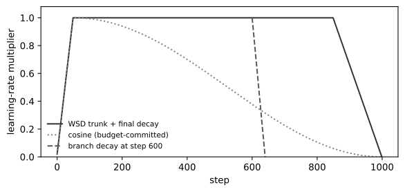
One honesty note, and it generalizes: a single-seed loss curve at toy scale cannot rank optimizers. A defensible optimizer claim needs paired seeds, learning-rate sweeps for both candidates, equal tokens, and the memory, communication, and stability bills priced alongside the loss — which is why this section taught mechanisms and ledger effects, and left leaderboards to the testbeds built for them.
6.8 Goodput, faults, and the checkpoint interval
MFU is measured while steps execute. It says nothing about the hours when steps do not execute — and at frontier scale those hours are the story. The Llama 3 405B training report counts 466 job interruptions over 54 days on a 16,384-GPU cluster, 419 of them unexpected, and about 78% of those hardware-related (Grattafiori et al. 2024). Goodput is the metric that refuses to look away: useful training progress per wall-clock hour, roughly MFU times the fraction of wall time spent actually training. A cluster at 45% MFU and 85% availability delivers 38% goodput; heroic kernel work that lifts MFU three points matters less than a checkpoint-and-recovery pipeline that lifts availability ten.
The tax has a structure. When a run fails, it loses (i) the work since the last checkpoint, (ii) the restart time, and it pays continuously (iii) the cost of writing checkpoints at all. Checkpoint too rarely and failures are catastrophic; too often and the writing is the catastrophe. For checkpoint cost C_s seconds, mean time between failures M, restart cost R, and interval I, the wasted fraction is approximately
w(I) = \frac{C_s}{I} + \frac{I}{2M} + \frac{R}{M}, \tag{6.5}
overhead plus expected lost work (failures land midway through an interval on average) plus restarts. Minimizing over I gives Young’s approximation (Young 1974):
I^{*} = \sqrt{2\,C_s\,M}. \tag{6.6}
Every input is something we can now compute. The checkpoint payload comes from our own ledger — weights, master weights, and moments; gradients need not persist. MTBF comes from the published failure data, scaled to cluster size: failures arrive per-device, so a cluster’s MTBF is the per-device MTBF divided by device count.
# @save
def checkpoint_waste(interval_s: float, save_s: float, mtbf_s: float, restart_s: float = 300.0) -> float:
    """Return the fraction of cluster time wasted by a checkpoint policy.

    Implements the classic three-term model: save overhead ``C_s / I``,
    expected lost work ``I / 2M`` (a failure lands midway through an
    interval on average), and restart cost ``R / M``. Valid when
    intervals are short against MTBF and failures arrive independently —
    correlated rack failures and preemption warnings break it, in the
    conservative direction.

    Args:
        interval_s: Seconds between checkpoint starts.
        save_s: Seconds of training stalled per synchronous save.
        mtbf_s: Mean seconds between job-interrupting failures.
        restart_s: Seconds to detect, reschedule, and reload.

    Returns:
        The wasted fraction of wall-clock time.
    """
    return save_s / interval_s + interval_s / (2 * mtbf_s) + restart_s / mtbf_s


def young_interval(save_s: float, mtbf_s: float) -> float:
    """Return Young's optimal checkpoint interval ``sqrt(2 * C_s * M)``."""
    return math.sqrt(2 * save_s * mtbf_s)
Feed it inputs computed from our own artifacts rather than assumed:
ledger = state_ledger(P_7B, "mixed")
payload = ledger["total"] - ledger["gradients"]
save_seconds = payload / (3 * GIB)  # illustrative 3 GiB/s effective write path
device_mtbf = 54 * 86_400 * 16_384 / 419  # per-device seconds, Llama 3 unexpected-failure rate
print(f"checkpoint payload {payload / GIB:.0f} GiB -> save stall {save_seconds:.0f} s; "
      f"per-device MTBF {device_mtbf / 86_400 / 365:.1f} device-years")
checkpoint payload 88 GiB -> save stall 29 s; per-device MTBF 5.8 device-yearsEighty-eight gibibytes per save, thirty seconds of stall, and a per-device MTBF of about six device-years — a number that sounds comfortable until you multiply by a fleet. Now the policy, computed for a 1,024-device version of our 7B run and for a Llama-scale 16,384-device job:
for devices in (1_024, 16_384):
    mtbf = device_mtbf / devices
    best = young_interval(save_seconds, mtbf)
    waste = checkpoint_waste(best, save_seconds, mtbf)
    print(f"{devices:6,} devices: cluster MTBF {mtbf / 3600:5.1f} h -> "
          f"checkpoint every {best / 60:4.0f} min, minimum waste {waste:.1%}")
1,024 devices: cluster MTBF 49.5 h -> checkpoint every 54 min, minimum waste 2.0%
16,384 devices: cluster MTBF 3.1 h -> checkpoint every 13 min, minimum waste 9.9%The same save cost yields opposite policies: the small cluster checkpoints hourly and wastes 2%, the large one must save every quarter hour and still burns 10% of everything it does — with Equation 6.5, failure math becomes a line item you can budget rather than a surprise. Figure 6.6 shows the useful shape of the curve: flat near the optimum (being 2x off costs little) and vicious at the too-rare end. This is also the economic argument for the engineering that changes the constants: asynchronous checkpointing stages state to host memory in seconds and drains to storage in the background, shrinking C_s tenfold, and Llama 3’s operations held effective training time above 90% on exactly such machinery (Grattafiori et al. 2024).
Show the code that draws this figure
intervals = [60 * m for m in range(1, 241)]
fig, ax = plt.subplots(figsize=(6.2, 3.2))
for devices, style in ((1_024, "-"), (16_384, "--")):
    mtbf = device_mtbf / devices
    ax.plot([i / 60 for i in intervals],
            [checkpoint_waste(i, save_seconds, mtbf) for i in intervals],
            style, color="0.3", label=f"{devices:,} devices")
    best = young_interval(save_seconds, mtbf)
    ax.plot(best / 60, checkpoint_waste(best, save_seconds, mtbf), "o", color="0.1", ms=5)
ax.set_xlabel("checkpoint interval (minutes)")
ax.set_ylabel("wasted fraction of cluster time")
ax.set_ylim(0, 0.30)
ax.legend(frameon=False, fontsize=8)
fig.tight_layout()
plt.show()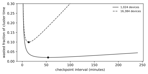
Two failure classes deserve names because checkpoints alone do not solve them. Silent data corruption — a device computing plausible wrong numbers without raising an error — evades every crash-triggered defense; fleets counter it with burn-in screens, periodic redundant-computation probes, and checksums on collectives, because restoring a checkpoint that was written from corrupted state just replays the corruption. And loss spikes — sudden optimization blow-ups from data anomalies, numerical range issues, or routing collapse in MoE models — require a diagnosis before a response: skip the batch if it is data, rescale if it is numerics, roll back to a verified checkpoint if the optimizer state itself went bad. A checkpoint is only a recovery point if what you saved was healthy, which is why frontier runs pair every save with cheap validation — finite-norm checks, a held-out loss probe — before marking it restorable.
6.9 From FLOPs to dollars to megawatts
Everything so far priced a run in bytes and seconds. The last conversion prices it in money and electricity, and it is shorter than its reputation: from Chapter 5, training compute is C \approx {6}ND FLOPs for N parameters and D tokens; a fleet of G devices with peak rate F_{\text{peak}} at utilization u delivers G F_{\text{peak}} u FLOPs per second; divide and convert. Device-hours, notably, do not depend on G at all —
H = \frac{6ND}{F_{\text{peak}}\, u \cdot 3600}, \qquad T_{\text{days}} = \frac{H}{24\,G}, \tag{6.7}
so buying more devices buys calendar time, never fewer device-hours; only u — the MFU-times-goodput product this chapter has been building — changes what the compute costs. Money is device-hours times a price; power is fleet size times per-device draw times the facility overhead factor PUE (total facility power over IT power, ~1.1–1.4). As code:
# @save
def run_economics(
    params: float, tokens: float, devices: int, *,
    peak_tflops: float = 989.0, mfu: float = 0.40, price_per_hour: float = 2.50,
    kw_per_device: float = 1.4, pue: float = 1.2,
) -> dict[str, float]:
    """Convert a training budget into hours, dollars, and megawatts.

    Applies the dense-Transformer estimate ``C = 6 N D``, divides by
    delivered FLOPs (peak times MFU) for device-hours, then prices time
    at an hourly rate and power at per-device draw times PUE. The
    defaults are illustrative 2026 H100-class planning constants — the
    dated landscape callout carries their provenance; the formulas are
    the durable part.

    Args:
        params: Trainable parameters ``N``.
        tokens: Training tokens ``D``.
        devices: Fleet size ``G`` (sets calendar time and megawatts).
        peak_tflops: Per-device peak TFLOP/s in training precision.
        mfu: Delivered fraction of peak (fold goodput in here too).
        price_per_hour: Effective all-in device-hour price in dollars.
        kw_per_device: Average IT draw per device including host share.
        pue: Facility power overhead factor (total / IT).

    Returns:
        FLOPs, device-hours, wall days, cost, megawatts, energy MWh,
        and dollars per million tokens, keyed by name.
    """
    flops = 6 * params * tokens
    device_hours = flops / (peak_tflops * 1e12 * mfu) / 3600
    wall_days = device_hours / devices / 24
    megawatts = devices * kw_per_device * pue / 1000
    return {
        "flops": flops, "device_hours": device_hours, "wall_days": wall_days,
        "cost": device_hours * price_per_hour, "megawatts": megawatts,
        "energy_mwh": megawatts * wall_days * 24,
        "usd_per_m_tokens": device_hours * price_per_hour / tokens * 1e6,
    }
We evaluate it for three named-scale runs — parameter and token budgets shaped like Llama 2 7B, Llama 3 70B, and Llama 3 405B, with fleet sizes in their reported ranges:
runs = [
    ("7B on 2T tokens", 6.74e9, 2.0e12, 1_024),
    ("70B on 15T tokens", 70.6e9, 15.0e12, 16_384),
    ("405B on 15.6T tokens", 405e9, 15.6e12, 16_384),
]
print("run                     FLOPs   device-hrs   days     cost     MW    energy")
for name, n, d, g in runs:
    eco = run_economics(n, d, g)
    print(f"{name:21s} {eco['flops']:8.1e} {eco['device_hours'] / 1e6:7.2f}M "
          f"{eco['wall_days']:6.1f} ${eco['cost'] / 1e6:6.1f}M {eco['megawatts']:6.1f} "
          f"{eco['energy_mwh']:7,.0f} MWh")
run FLOPs device-hrs days cost MW energy
7B on 2T tokens 8.1e+22 0.06M 2.3 $ 0.1M 1.7 95 MWh
70B on 15T tokens 6.4e+24 4.46M 11.3 $ 11.2M 27.5 7,495 MWh
405B on 15.6T tokens 3.8e+25 26.62M 67.7 $ 66.5M 27.5 44,718 MWhThree sanity checks make these more than pretty rows. The 405B estimate of 26.6M device-hours sits within 15% of the 30.84M H100-hours Meta reported for that run (Grattafiori et al. 2024) — our 40% MFU assumption is slightly generous and {6}ND ignores attention FLOPs, both in the expected direction. The 27.5 MW line explains why frontier training is now an energy story: one pretraining run holds the power draw of a small town for two months, and the 100-megawatt-class campuses being built are this row multiplied by concurrent runs and headroom. And the middle column repeats Equation 6.7’s lesson: the 70B and 405B runs use the same fleet, so their dollar gap is purely device-hours — scale bought time, not efficiency.
Renting at $2.50 per device-hour is one side of a decision; the other is owning. Ownership converts a capital price into an hourly cost through the capital recovery factor — the annuity formula that spreads principal plus return over a useful life —
\operatorname{CRF} = \frac{r\,(1+r)^{L}}{(1+r)^{L} - 1}, \tag{6.8}
for discount rate r and life L years: annualized cost equals CRF times the capital outlay, and the effective hourly rate divides by the hours you actually use.
# @save
def capital_recovery_factor(rate: float, years: int) -> float:
    """Return the annuity factor that annualizes a capital purchase.

    Multiplying a purchase price by the CRF gives the constant annual
    payment that repays principal plus the required return over the
    asset's life — the standard way to put "buy a cluster" and "rent by
    the hour" in the same units.

    Args:
        rate: Annual discount rate (0.12 means twelve percent).
        years: Useful life in years.

    Returns:
        The annual payment per dollar of capital.
    """
    growth = (1 + rate) ** years
    return rate * growth / (growth - 1)
At a 12% discount rate over a four-year life, with an illustrative all-in system price of $45k per installed device and energy at eight cents per kWh:
crf = capital_recovery_factor(0.12, 4)
system_cost, energy_at_full = 45_000.0, 1.4 * 1.2 * 8_766 * 0.08
annualized = crf * system_cost
print(f"CRF(12%, 4y) = {crf:.4f} -> ${annualized:,.0f}/device-year plus ${energy_at_full:,.0f} energy")
for utilization in (0.95, 0.70, 0.40):
    hourly = (annualized + energy_at_full * utilization) / (8_766 * utilization)
    print(f"  at {utilization:.0%} utilization: effective ${hourly:4.2f}/device-hour")
CRF(12%, 4y) = 0.3292 -> $14,816/device-year plus $1,178 energy
at 95% utilization: effective $1.91/device-hour
at 70% utilization: effective $2.55/device-hour
at 40% utilization: effective $4.36/device-hourThe whole rent-versus-buy argument is in those three lines: ownership at $45k per installed device beats the $2.50 rental only above roughly 70% sustained utilization — and utilization is a schedule-and-operations achievement, not a purchase. A cluster bought for one training burst then idling between runs costs more per useful hour than the cloud it was meant to undercut; conversely, a continuously-scheduled fleet (training, then Chapter 10 serving, then experiments) clears the bar easily. The full decision adds terms the formula omits — time-to-capacity while a cluster is built, topology guarantees rented clouds may not give, resale and technology-stranding risk on a four-year-old SKU — but the CRF frame forces each to be priced as a utilization or rate adjustment instead of argued as vibes. Figure 6.7 closes the loop from FLOPs to facilities.
Show the code that draws this figure
names = [name for name, *_ in runs]
econ = [run_economics(n, d, g) for _, n, d, g in runs]
fig, (left, right) = plt.subplots(1, 2, figsize=(6.8, 3.0))
cost_bars = left.bar(range(3), [e["cost"] / 1e6 for e in econ], color="0.45", width=0.55)
left.bar_label(cost_bars, fmt="$%.1fM", padding=2, fontsize=8)
left.set_yscale("log")
left.set_ylabel("compute cost (million USD, log)")
left.set_ylim(0.05, 200)
mw_bars = right.bar(range(3), [e["megawatts"] for e in econ], color="0.65", width=0.55)
right.bar_label(mw_bars, fmt="%.1f MW", padding=2, fontsize=8)
right.set_ylabel("facility power (MW)")
for ax in (left, right):
    ax.set_xticks(range(3), ["7B\n2T", "70B\n15T", "405B\n15.6T"], fontsize=8)
fig.tight_layout()
plt.show()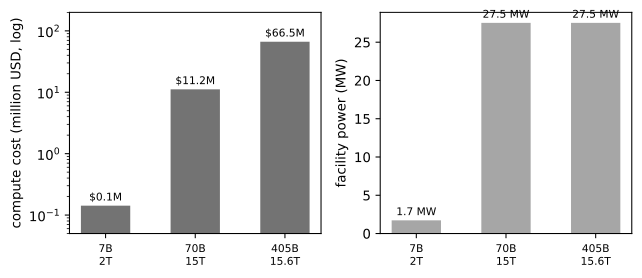
Note
Landscape 2026 (dated). The constants behind this section’s cells, verified 2026-07-20, are planning-grade illustrations, not quotes. Per-device peak: 989 TFLOP/s is H100-class dense BF16; current-generation parts (NVIDIA GB300/Blackwell-Ultra-class, with the Vera Rubin platform announced; Google Ironwood TPUs; AMD MI350-series) quote several-fold higher peaks under new sparsity and FP4/FP8 conventions that are not directly comparable — always match the dtype and density of your actual recipe. Prices: roughly $2–3 per H100-hour at neoclouds (CoreWeave, Lambda, Nebius and peers, whose GPU-first data centers and willingness to sign short commitments undercut hyperscaler list prices of $4–6), with frontier labs instead signing multi-year power-and-capacity deals measured in gigawatts and billions of dollars. Power: ~0.7–1.4 kW per device including host share, PUE 1.1–1.4. FP8 pretraining recipes in the DeepSeek-V3 lineage and OCP microscaling formats (MX, NVFP4) are current low-precision practice; Muon-class optimizers now appear in production-scale reports and a PyTorch API. The US 1e26-FLOP reporting threshold of Executive Order 14110 was revoked in January 2025 and has no active general successor as of this date — compute-threshold governance survives as policy proposals and state law, covered with the rest of the governance surface in Chapter 25. Verify live: Epoch AI’s training-cost analyses, vendor spec sheets for your actual SKU and dtype, and two current cloud quotes before any decision that spends money.
6.10 Summary
We priced a training step from shapes alone: a 7B model carries 100 GiB of optimizer-visible state — identical under fp32 and mixed precision — plus activations spanning two orders of magnitude across saving policies, a range we confirmed by measuring what autograd stores. ZeRO shards the state; tensor and pipeline parallelism split the computation, and our simulator showed composition flipping from “just use data parallelism” at 7B to “model parallelism is forced” at 70B. We measured an honest toy MFU, computed the checkpoint interval failure rates dictate, and converted FLOPs to dollars and megawatts within 15% of a published frontier run. Chapter 7 turns to what those FLOPs buy next: post-training.
6.11 Exercises
- Re-price the optimizer. Add an
"adam8bit"recipe toPRECISION_RECIPES(one byte per moment plus 0.5 bytes of block-scale metadata, master weights unchanged) and a"muon"recipe (four-byte momentum, no second moment, master weights unchanged). Recompute the ZeRO-1 table of Section 6.3 for both at 8 and 64 shards. At which sharding degree does the recipe choice stop mattering for feasibility on an 80 GiB device, and why does sharding erode the advantage? - Find the checkpointing crossover. Using
activation_bytes_per_layerand the {\approx}\,1/3 extra-compute cost of full recomputation, compute the sequence length at which the 7B configuration must checkpoint (activations alone exceed an 80 GiB device under the fused-attention policy) at microbatch 1. Then userun_economicsto price the recomputation tax in dollars for the 7B-on-2T run. Is checkpointing ever worth it when the memory does fit? - Stress the plan simulator.
- Rerun
plan_tablefor the 70B configuration withzero_stage=3and explain every feasibility verdict that changes. - Double the global batch to 256 and identify which pipeline-heavy plans become competitive purely through bubble amortization.
- Add a
context_parallelaxis toevaluate_planthat dividesseq_lenacross devices and multiplies device count; verify that atseq_len=131_072no plan without it fits the 70B model.
- Rerun
- Break the pipeline’s balance. Extend
simulate_pipelineso one chosen stage runs 1.3x slower than the rest (a straggler or an unbalanced layer split). Measure the idle fraction for S=8, m=32 and compare it to Equation 6.3’s prediction. How much imbalance makes the straggler term dominate the fill-and-drain term? - Interrogate the MFU denominator. Sweep
measured_matmul_flopsover n \in \{256, 512, 1024, 2048\} and recompute the toy MFU against each roofline. The model’s “utilization” changes while the training loop does not move — state precisely what claim an MFU number makes, and which denominator convention a skeptical reader should demand alongside any published figure. - Checkpoint under preemption. Spot-market capacity often delivers a warning (say, 30 seconds) before reclaiming a node — enough to trigger one emergency save. Extend
checkpoint_wastewith a warned-preemption fraction p whose failures lose no work but still pay C_s + R, and recompute the optimal interval for the 16,384-device case at p \in \{0.5, 0.9\}. At what p does the periodic checkpoint schedule stop mattering? - Defend rent-versus-buy to a CFO. Your team proposes buying 1,024 devices for the 7B-class run and its successors. Using
run_economicsandcapital_recovery_factor, produce: the break-even sustained utilization against your current rental rate; the sensitivity of that break-even to a 2x energy-price change and to a three-year rather than four-year life; and the three operational observations from this chapter (not financial ones) that would most change the recommendation. State which inputs are measurements and which are assumptions.