# @save
from __future__ import annotations

import hashlib
import json
import math
import random
import sqlite3
from dataclasses import dataclass
from heapq import heappop, heappush
from itertools import count


def posterior(prior: float, sensitivity: float, false_positive: float) -> float:
    """Return the posterior probability of a condition given a positive test.

    Applies Bayes' rule to a binary detector. The point of the exercise is that
    a rare condition stays rare even after a positive result, because the flood
    of false positives from the large negative population swamps the true ones.

    Args:
        prior: Base rate of the condition before any test.
        sensitivity: P(test positive | condition present).
        false_positive: P(test positive | condition absent).

    Returns:
        P(condition present | test positive), between zero and one.
    """

    hit = sensitivity * prior
return hit / (hit + false_positive * (1 - prior))Appendix A — The Bridge: Math, Decisions, Planning, RL, Control, and Systems
This appendix is a bridge, not a compressed degree program. The spine assumes neural-network fundamentals; agent engineering also borrows from probability, decision theory, causal inference, optimization, planning, reinforcement learning, control, distributed systems, and security. Rather than re-teach each field, we carry across exactly what the chapters consume: for every topic, one worked calculation you can run, one picture, and the design-review question it lets you ask. Read a section when a chapter points here, and stop when that chapter reads again. Every number below is produced by the code on the page, not asserted.
Use this map to find only the bridge you need.
| Bridge section | Consumed by | What stalls if skipped |
|---|---|---|
| probability and information | Chapters 2, 7, 9, 22 | cross-entropy, KL, entropy, calibration |
| decision theory | Chapters 9, 16, 22, 28 | abstention, clarifying questions, asymmetric harm |
| causal inference | Chapters 22, 27 | logged-policy evaluation, canaries, confounding |
| constrained optimization | Chapters 1, 22, 26, 28 | safety constraints, Pareto choices, agency budgets |
| search and symbolic planning | Chapters 8, 16, 21, 31 | A*, MCTS, verifiers, explicit plans |
| sequential decisions / RL | Chapters 16, 23, 28, 31 | MDP, POMDP, belief, regret, exploration |
| control theory | Chapters 16, 17, 26, 27 | feedback, lag, instability, deadbands |
| distributed systems | Chapters 17, 26, 27 | partial failure, idempotency, queues, retries |
| threat modeling | Chapters 17, 24, 26 | assets, trust boundaries, attack paths |
The target depth is one worked calculation and the right design-review question. Where a chapter owns the deeper application, this bridge points to it: it defines an MDP, for instance, but Chapter 23 trains the agent; it prices a clarifying question, but Chapter 9 owns abstention.
A.1 Probability and information theory
Probability represents uncertainty about events. For event A, P(A) lies between zero and one, and conditional probability P(A \mid B) = P(A \cap B)/P(B) asks how belief about A changes after observing B. Bayes’ rule reverses the conditional:
P(A \mid B) = \frac{P(B \mid A)\,P(A)}{P(B)}.
The single most useful consequence is that a positive test result rarely means the tested-for thing is present, because base rates dominate. Suppose two percent of requests contain abuse, and a detector has ninety percent sensitivity with a five percent false-positive rate. We compute the posterior directly rather than trusting intuition.
Running it on the abuse detector:
print(f"P(abuse | +) = {posterior(0.02, 0.90, 0.05):.3f}")P(abuse | +) = 0.269A positive raises risk from two percent to about twenty-seven percent — real evidence, but not proof. Figure A.1 shows why: out of a thousand requests, the eighteen true positives are outnumbered by forty-nine false positives, so most alarms are false even with a good detector. The same arithmetic governs anomaly detection, guardrail classifiers, and alert triage; a chapter that quotes “ninety-five percent accuracy” without a base rate has not yet said anything about how many alarms will be real.
Show the code that draws this figure
import matplotlib.pyplot as plt

n = 1000
abuse = round(n * 0.02)
tp = round(abuse * 0.90)
fp = round((n - abuse) * 0.05)
fig, ax = plt.subplots(figsize=(6.2, 1.9))
ax.barh(0, tp, color="#c0392b", label=f"true positive ({tp})")
ax.barh(0, fp, left=tp, color="#e59866", label=f"false positive ({fp})")
ax.barh(1, abuse - tp, color="#7f8c8d", label=f"missed abuse ({abuse - tp})")
ax.set_yticks([0, 1])
ax.set_yticklabels(["alarms", "missed"])
ax.set_xlabel("requests (of 1000)")
ax.legend(loc="lower right", fontsize=8)
ax.spines[["top", "right"]].set_visible(False)
fig.tight_layout()
plt.show()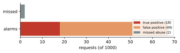
Information theory measures uncertainty itself. For a discrete distribution p, entropy H(p) = -\sum_x p(x)\log p(x) is expected surprise: highest when mass is spread evenly, lowest when one outcome dominates. Cross-entropy H(p, q) = -\sum_x p(x)\log q(x) scores a prediction q against data p, and Kullback–Leibler divergence D_{\mathrm{KL}}(p \Vert q) = \sum_x p(x)\log\frac{p(x)}{q(x)} is the extra cost of using q when the data follow p. KL is nonnegative but not symmetric, which is why it is a divergence and not a distance.
# @save
def entropy(dist: list[float]) -> float:
    """Return the Shannon entropy of a distribution, in bits.

    Args:
        dist: Probabilities that sum to one.

    Returns:
        Expected surprise in bits; larger means less predictable.
    """

    return -sum(p * math.log2(p) for p in dist if p > 0)


def kl_divergence(p: list[float], q: list[float]) -> float:
    """Return KL(p || q) in bits, the coding penalty for modelling p as q.

    The two orderings differ because KL punishes putting little q-mass where p
    has mass far more than the reverse; swapping the arguments is not a rounding
    detail but a different question.

    Args:
        p: The true distribution (the expectation is taken under it).
        q: The model distribution being charged for.

    Returns:
        A nonnegative divergence in bits, zero only when p equals q.
    """

    return sum(pi * math.log2(pi / qi) for pi, qi in zip(p, q) if pi > 0)
We show all three on a peaked and a uniform three-way distribution:
peaked, uniform = [0.90, 0.05, 0.05], [1 / 3, 1 / 3, 1 / 3]
print(f"H(peaked)  = {entropy(peaked):.3f} bits")
print(f"H(uniform) = {entropy(uniform):.3f} bits")
print(f"D(peaked || uniform) = {kl_divergence(peaked, uniform):.3f} bits")
print(f"D(uniform || peaked) = {kl_divergence(uniform, peaked):.3f} bits")
H(peaked) = 0.569 bits
H(uniform) = 1.585 bits
D(peaked || uniform) = 1.016 bits
D(uniform || peaked) = 1.347 bitsThe uniform distribution carries the full 1.585 bits a three-way choice can hold; the peaked one carries about a third of that. And the two KL values, 1.016 and 1.347, are genuinely different — the asymmetry is real, which matters in Chapter 7, where KL is a leash between a post-trained policy and its reference and the direction of the leash is a design choice. Cross-entropy is also the language-model loss: for one observed target token it reduces to the negative log probability the model assigned that token, and averaging that over training tokens is exactly the objective Chapter 2 minimizes.
A.2 Statistical decision theory
A probability describes belief; a decision combines belief with consequences. Given state s, action a, and loss L(a, s), the Bayes action minimizes expected loss, a^* = \arg\min_a \mathbb{E}_{s}[L(a, s)]. This is why one confidence threshold cannot serve every action: the loss, not the probability, decides. Chapter 1 makes the same move when it turns an uncertain answer into an abstention; here we price it.
Take the support-ticket example. An urgent ticket has probability 0.2 of being urgent; escalating an ordinary ticket costs one unit of operator time, and failing to escalate an urgent one costs ten.
# @save
def best_expected_loss(p_urgent: float, false_negative: float, false_positive: float) -> float:
    """Return the loss of the better of two actions under asymmetric costs.

    Compares *escalate* (which risks a false positive) against *do not escalate*
    (which risks a false negative) and returns whichever expected loss is
    smaller. Asymmetric costs, not the raw probability, choose the action.

    Args:
        p_urgent: Probability the ticket is genuinely urgent.
        false_negative: Cost of failing to escalate an urgent ticket.
        false_positive: Cost of escalating an ordinary ticket.

    Returns:
        The minimum expected loss across the two actions.
    """

    escalate = (1 - p_urgent) * false_positive
    do_not = p_urgent * false_negative
return min(escalate, do_not)print(f"R(escalate) = {(1 - 0.2) * 1:.2f}")
print(f"R(do not) = {0.2 * 10:.2f}")
print(f"best loss = {best_expected_loss(0.2, 10, 1):.2f} (escalate)")R(escalate) = 0.80
R(do not) = 2.00
best loss = 0.80 (escalate)Escalation wins despite the low urgent probability, because the loss is asymmetric. Figure A.2 turns the two numbers into a threshold: the escalate and do-not-escalate lines cross at the urgency probability where (1 - p) = 10p, that is at about 0.091. Below it, ignore; above it, escalate. The design question is not “how confident is the model?” but “where is the crossover, given our costs?”
Show the code that draws this figure
import matplotlib.pyplot as plt

ps = [i / 100 for i in range(101)]
fig, ax = plt.subplots(figsize=(6.2, 3.0))
ax.plot(ps, [(1 - p) * 1 for p in ps], label="escalate (risk false positive)")
ax.plot(ps, [p * 10 for p in ps], label="do not escalate (risk false negative)")
ax.axvline(1 / 11, ls=":", color="0.5")
ax.set_xlabel("P(urgent)")
ax.set_ylabel("expected loss")
ax.set_ylim(0, 2.2)
ax.legend(fontsize=8)
ax.spines[["top", "right"]].set_visible(False)
fig.tight_layout()
plt.show()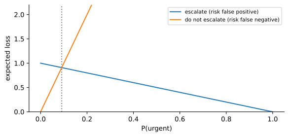
An observation has value of information (VOI) when it can change the action and lower expected loss. The value before paying for the observation is never negative, because the decision-maker can always ignore what it learns. We evaluate one binary signal — a classifier with a sensitivity and a specificity — and print not just the final VOI but the two posteriors that produce it, so the mechanism is visible rather than trusted.
# @save
def value_of_signal(
    prior_urgent: float,
    sensitivity: float,
    specificity: float,
    false_negative: float,
    false_positive: float,
) -> dict[str, float]:
    """Return the expected loss a single binary observation avoids.

    Splits the world into signal-positive and signal-negative, updates the
    urgency belief in each branch by Bayes' rule, takes the best action within
    each branch, and reports the reduction in expected loss versus deciding now.
    The result is nonnegative: information cannot hurt a decision-maker free to
    ignore it. Compare it against the money, latency, and friction of asking.

    Args:
        prior_urgent: Belief the ticket is urgent before the signal.
        sensitivity: P(signal positive | urgent).
        specificity: P(signal negative | not urgent).
        false_negative: Cost of missing an urgent ticket.
        false_positive: Cost of escalating an ordinary one.

    Returns:
        A dict with the prior loss, P(positive), the two branch posteriors, and
        the value of information itself.
    """

    prior_loss = best_expected_loss(prior_urgent, false_negative, false_positive)
    p_pos = prior_urgent * sensitivity + (1 - prior_urgent) * (1 - specificity)
    post_pos = prior_urgent * sensitivity / p_pos
    post_neg = prior_urgent * (1 - sensitivity) / (1 - p_pos)
    observed = p_pos * best_expected_loss(post_pos, false_negative, false_positive) + (
        1 - p_pos
    ) * best_expected_loss(post_neg, false_negative, false_positive)
    return {
        "prior_loss": prior_loss,
        "p_positive": p_pos,
        "posterior_positive": post_pos,
        "posterior_negative": post_neg,
        "voi": prior_loss - observed,
    }
for name, value in value_of_signal(0.2, 0.85, 0.9, 10.0, 1.0).items():
print(f"{name:20s} {value:.3f}")prior_loss 0.800
p_positive 0.250
posterior_positive 0.680
posterior_negative 0.040
voi 0.420A positive signal lifts the urgency belief to 0.68 and a negative one drops it to 0.04, and averaging the best action in each branch avoids 0.42 loss units versus deciding now. That number is the price ceiling: ask the clarifying question, or run the extra classifier, only when its total cost — money, latency, privacy, user friction — is below 0.42. VOI is what gives an agent’s clarifying questions a principled trigger, and Chapter 9 turns it into abstention policy.
Finally, we need to score probabilistic forecasts honestly. A proper scoring rule is minimized in expectation by reporting your true belief. The Brier loss (p - y)^2 and the log loss -[y\log p + (1-y)\log(1-p)] are both proper; thresholded accuracy is not.
# @save
def brier(p: float, y: int) -> float:
    """Return the Brier score (p - y)^2 for probability p and outcome y."""

    return (p - y) ** 2


def log_loss(p: float, y: int) -> float:
    """Return the log loss for probability p and binary outcome y."""

    return -(y * math.log(p) + (1 - y) * math.log(1 - p))
We confirm properness by holding the true probability at 0.3 and varying the report:
true_p = 0.3
for report in (0.3, 0.5, 0.1):
    e_brier = true_p * brier(report, 1) + (1 - true_p) * brier(report, 0)
    e_log = true_p * log_loss(report, 1) + (1 - true_p) * log_loss(report, 0)
    print(f"report={report}: E[Brier]={e_brier:.4f}  E[log]={e_log:.4f}")
report=0.3: E[Brier]=0.2100 E[log]=0.6109
report=0.5: E[Brier]=0.2500 E[log]=0.6931
report=0.1: E[Brier]=0.2500 E[log]=0.7645The honest report, 0.3, minimizes both expected scores; the overconfident 0.1 and the hedged 0.5 are strictly worse. That is what “proper” buys, and it is why Chapter 22 grades judges and risk estimates with proper scores rather than accuracy, which can reward a forecaster for hiding uncertainty. The distinction between aleatoric uncertainty (irreducible outcome noise) and epistemic uncertainty (reducible by evidence) rides on the same machinery: only epistemic uncertainty can be bought down, and VOI is how you decide whether the purchase is worth it.
A.3 Causal inference for evaluation
Prediction asks what co-occurs; causal inference asks what would change under an intervention. The distinction bites whenever the deployed policy affects which data you observe — which is every canary, every A/B test on a routed system, every evaluation of a policy from its own logs. Figure A.3 draws the trap: task difficulty D raises both the chance a ticket is routed to a new agent A and the chance it fails to resolve Y, so difficulty is a confounder — a common cause opening a backdoor path A \leftarrow D \rightarrow Y that a naive comparison mistakes for the agent’s effect.
flowchart LR
    D["Difficulty D<br/>(confounder)"] --> A["Routed to new agent A"]
    D --> Y["Resolved Y"]
    A -->|"effect we want"| Y
We make the trap numeric. Generate synthetic logs where hard tickets are preferentially routed to the new agent, and where the agent’s true causal effect is a constant plus-ten points of resolution regardless of difficulty. A naive difference of outcome rates should be badly wrong; a difficulty-adjusted estimate should recover the truth.
# @save
def simulate_routing(n: int, seed: int) -> list[tuple[str, int, int]]:
    """Return synthetic (difficulty, action, outcome) logs with confounding.

    Hard tickets are routed to the new agent far more often than easy ones, so
    difficulty is a common cause of treatment and outcome. The new agent's true
    causal effect is a constant +0.10 on resolution probability at every
    difficulty; the confounding is what a naive comparison will get wrong.

    Args:
        n: Number of logged tickets to generate.
        seed: Seed for the deterministic pseudo-random stream.

    Returns:
        A list of (difficulty, action, outcome) triples.
    """

    rng = random.Random(seed)
    route = {"easy": 0.2, "hard": 0.8}
    resolve = {("easy", 0): 0.8, ("easy", 1): 0.9, ("hard", 0): 0.3, ("hard", 1): 0.4}
    rows = []
    for _ in range(n):
        d = "hard" if rng.random() < 0.5 else "easy"
        a = 1 if rng.random() < route[d] else 0
        y = 1 if rng.random() < resolve[(d, a)] else 0
        rows.append((d, a, y))
    return rows


def _rate(rows: list[tuple[str, int, int]]) -> float:
    return sum(y for *_, y in rows) / len(rows)


def naive_effect(rows: list[tuple[str, int, int]]) -> float:
    """Return P(Y|A=1) - P(Y|A=0), the confounded difference of outcome rates."""

    return _rate([r for r in rows if r[1] == 1]) - _rate([r for r in rows if r[1] == 0])


def backdoor_effect(rows: list[tuple[str, int, int]]) -> float:
    """Return the difficulty-adjusted effect, averaging within each stratum.

    Implements backdoor adjustment: estimate the treatment effect separately
    within each level of the confounder D, then average by the prevalence of D.
    Because D no longer varies within a stratum, it can no longer masquerade as
    the agent's effect.

    Args:
        rows: Logged (difficulty, action, outcome) triples.

    Returns:
        The confounding-adjusted estimate of the causal effect.
    """

    effect = 0.0
    for d in ("easy", "hard"):
        stratum = [r for r in rows if r[0] == d]
        weight = len(stratum) / len(rows)
        treated = [r for r in stratum if r[1] == 1]
        control = [r for r in stratum if r[1] == 0]
        effect += weight * (_rate(treated) - _rate(control))
    return effect
logs = simulate_routing(20_000, seed=0)
print(f"naive difference = {naive_effect(logs):+.3f} (looks like the agent is worse)")
print(f"backdoor-adjusted = {backdoor_effect(logs):+.3f} (true effect is +0.100)")naive difference = -0.202 (looks like the agent is worse)
backdoor-adjusted = +0.091 (true effect is +0.100)The naive difference says the new agent is twenty points worse; the adjusted estimate says it is ten points better. The confounder did not merely add noise — it flipped the sign. That is the whole reason Chapter 27 refuses to trust a raw before-and-after comparison when routing, region, or risk changed exposure. The backdoor criterion names the rule: adjust for a set of observed variables that blocks every noncausal path into treatment, and do not adjust mechanically for everything, because conditioning on a collider or a post-treatment variable opens bias rather than closing it. Draw the graph first.
Backdoor adjustment needs the confounder measured. The frontdoor criterion is its escape hatch: when an unmeasured confounder blocks the backdoor, but the treatment acts only through a fully observed mediator M (so A \rightarrow M \rightarrow Y) that the confounder does not touch, the effect is still identified by chaining A \rightarrow M and M \rightarrow Y. It is rare in practice because a clean, complete mediator is a strong assumption, but it is the reason “we can’t randomize” is not automatically “we can’t identify.”
When we cannot adjust because the logs came from a different policy, we reweight. Inverse propensity scoring estimates the value of a target policy \pi from logs drawn by a behavior policy \mu by weighting each reward by \pi(a\mid x)/\mu(a\mid x).
# @save
def ips_value(logged: list[tuple[int, float, float]]) -> float:
    """Return the inverse-propensity estimate of an always-treat policy.

    Each logged row is (action, reward, behavior-probability). The target policy
    always takes action 1, so rows where it disagrees drop out and surviving
    rows are up-weighted by the inverse of how likely the logging policy was to
    take that action. Rare actions get large weights, which is exactly why the
    estimator has high variance and can exceed the reward range on small logs.

    Args:
        logged: (action, reward, mu) triples from the behavior policy.

    Returns:
        The IPS estimate of the target policy's mean reward.
    """

    return sum((1.0 if a == 1 else 0.0) / mu * r for a, r, mu in logged) / len(logged)
logged = [(1, 1.0, 0.2), (0, 1.0, 0.8), (1, 0.0, 0.8), (0, 0.0, 0.2), (1, 1.0, 0.8)]
print(f"V_IPS(always-treat) = {ips_value(logged):.3f}")V_IPS(always-treat) = 1.250The estimate, 1.25, sits above the reward range of the data — a signal, not a bug: one rare treated action carried a large weight, and IPS is unbiased only when the behavior policy had overlap (nonzero probability of every action the target takes) and only useful when the weights stay small. The doubly robust estimator combines this reweighting with a learned outcome model and stays consistent if either the propensities or the outcome model is right; neither trick rescues unmeasured confounding or missing overlap. Chapter 22 owns off-policy evaluation; this bridge supplies the reason a naive log replay can lie.
A.4 Constrained and multi-objective optimization
Agent systems optimize several objectives at once: task quality, policy compliance, latency, cost, and operator load. Collapsing them to one blended score too early hides structure. A constrained problem keeps some objectives as inequalities — \min_\theta f(\theta) subject to g_j(\theta) \le 0 — and a hard constraint declares an infeasible region rather than a price. A penalty f(\theta) + \lambda \max(0, g(\theta)) softens the wall, useful during optimization but no substitute for a launch invariant: an excellent average score cannot buy back one cross-tenant disclosure.
With multiple objectives and no constraint to collapse them, configuration a dominates b when it is no worse on every objective and strictly better on at least one. The non-dominated set is the Pareto frontier, and everything behind it should leave consideration before anyone argues about preference weights. We compute the frontier over six illustrative model configurations rather than eyeballing a plot.
# @save
POINTS = {
    "small/direct": (1.0, 0.72),
    "small/RAG": (1.8, 0.83),
    "medium/direct": (2.8, 0.82),
    "medium/RAG": (3.6, 0.91),
    "large/agent": (7.2, 0.93),
    "large/ensemble": (11.0, 0.935),
}


def pareto_names(points: dict[str, tuple[float, float]]) -> set[str]:
    """Return the configurations no cheaper, no-worse point dominates.

    A point is dominated when some other point costs no more and scores no less,
    strictly beating it on at least one axis. The survivors form the Pareto
    frontier — the only candidates worth weighing preferences over, since a
    dominated point is beaten outright.

    Args:
        points: Name to (cost, quality); lower cost and higher quality are better.

    Returns:
        The set of non-dominated configuration names.
    """

    frontier = set()
    for name, (cost, quality) in points.items():
        dominated = any(
            oc <= cost and oq >= quality and (oc < cost or oq > quality)
            for other, (oc, oq) in points.items()
            if other != name
        )
        if not dominated:
            frontier.add(name)
return frontierprint("frontier :", sorted(pareto_names(POINTS)))
print("dominated:", sorted(set(POINTS) - pareto_names(POINTS)))frontier : ['large/agent', 'large/ensemble', 'medium/RAG', 'small/RAG', 'small/direct']
dominated: ['medium/direct']Exactly one configuration falls out: medium/direct is dominated because small/RAG costs less and scores higher, so it never deserves a preference discussion. Figure A.4 plots the survivors. A weighted sum \sum_j w_j f_j(\theta) is convenient but hides the units and stakeholder judgments inside the weights, and it can skip points on a non-convex frontier entirely. Use explicit constraints for non-negotiable limits, Pareto analysis for genuine tradeoffs, and lexicographic ordering when one objective truly dominates — discard everything that violates safety, then meet quality, then minimize cost. The design-review question is not “what is our score?” but “which constraints define feasibility, which points are dominated, and who owns preference among the rest?”
Show the code that draws this figure
import matplotlib.pyplot as plt

frontier = pareto_names(POINTS)
fig, ax = plt.subplots(figsize=(6.6, 3.6))
for name, (cost, quality) in POINTS.items():
    on = name in frontier
    ax.scatter(cost, quality, s=70, marker="o" if on else "x",
               color="#2f855a" if on else "#a0a0a0")
    ax.annotate(name, (cost, quality), xytext=(5, 5), textcoords="offset points", fontsize=8)
line = sorted(POINTS[n] for n in frontier)
ax.plot([c for c, _ in line], [q for _, q in line], color="#2f855a", lw=1.4)
ax.set_xlabel("illustrative cost per task (cents)")
ax.set_ylabel("task-and-policy success")
ax.set_ylim(0.65, 0.97)
ax.spines[["top", "right"]].set_visible(False)
fig.tight_layout()
plt.show()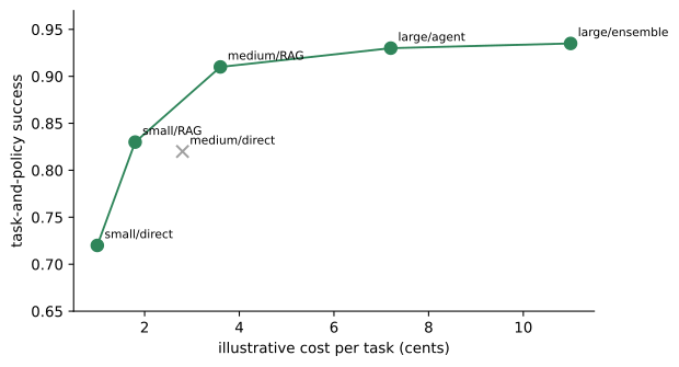
A.5 Classical search, planning, and symbolic reasoning
Language models propose plans; classical methods still supply the representations and the guarantees. A* searches a graph by expanding the node with the smallest f(n) = g(n) + h(n), where g(n) is the cost paid to reach n and h(n) estimates the cost remaining. When h never overestimates the true remaining cost — an admissible heuristic — A* returns an optimal path, and the more accurate h is, the fewer nodes it expands. We run it on a small grid with walls, using Manhattan distance as the heuristic, and count expansions against uninformed search.
# @save
GRID = ["S....", ".###.", ".#...", ".#.#.", "...#G"]


def _cell(mark: str) -> tuple[int, int]:
    return next((r, c) for r, row in enumerate(GRID) for c, ch in enumerate(row) if ch == mark)


def _neighbors(cell: tuple[int, int]):
    r, c = cell
    for dr, dc in ((-1, 0), (1, 0), (0, -1), (0, 1)):
        nr, nc = r + dr, c + dc
        if 0 <= nr < len(GRID) and 0 <= nc < len(GRID[0]) and GRID[nr][nc] != "#":
            yield (nr, nc)


def manhattan(a: tuple[int, int], b: tuple[int, int]) -> int:
    """Return the grid (L1) distance, an admissible heuristic for 4-connected moves."""

    return abs(a[0] - b[0]) + abs(a[1] - b[1])


def astar(heuristic) -> tuple[list, list]:
    """Return the optimal grid path and the cells expanded to find it.

    Expands the frontier node of least f = g + h until the goal is reached, then
    reconstructs the path from the recorded predecessors. The heuristic argument
    lets us compare an informed search (Manhattan distance) against uninformed
    search (a zero heuristic, which is Dijkstra) by counting expansions.

    Args:
        heuristic: A function from (cell, goal) to an optimistic cost estimate.

    Returns:
        A (path, expanded) pair: the start-to-goal cells and the expansion order.
    """

    start, goal = _cell("S"), _cell("G")
    tie = count()
    frontier = [(heuristic(start, goal), next(tie), start)]
    g_cost = {start: 0}
    came: dict[tuple[int, int], tuple[int, int]] = {}
    expanded: list[tuple[int, int]] = []
    while frontier:
        _, _, cell = heappop(frontier)
        if cell in expanded:
            continue
        expanded.append(cell)
        if cell == goal:
            break
        for nb in _neighbors(cell):
            step = g_cost[cell] + 1
            if step < g_cost.get(nb, math.inf):
                g_cost[nb] = step
                came[nb] = cell
                heappush(frontier, (step + heuristic(nb, goal), next(tie), nb))
    path = [goal]
    while path[-1] != start:
        path.append(came[path[-1]])
    return path[::-1], expanded
informed_path, informed_seen = astar(manhattan)
_, blind_seen = astar(lambda a, b: 0)
print(f"path length = {len(informed_path) - 1} steps")
print(f"A* expanded = {len(informed_seen)} cells")
print(f"Dijkstra expanded = {len(blind_seen)} cells (h = 0)")path length = 8 steps
A* expanded = 15 cells
Dijkstra expanded = 18 cells (h = 0)Both searches find an eight-step optimal path, but the heuristic lets A* skip three of the eighteen cells Dijkstra opens by pulling the frontier toward the goal. Figure A.5 shows the route threading the walls. The lesson the agent spine consumes is division of labor: a model can propose successors or a heuristic, while deterministic code preserves legality and cost accounting — the guarantee lives in the search, not the suggestion.
Show the code that draws this figure
import matplotlib.pyplot as plt

fig, ax = plt.subplots(figsize=(3.4, 3.4))
path_set = set(informed_path)
for r, row in enumerate(GRID):
    for c, ch in enumerate(row):
        if ch == "#":
            color = "#222222"
        elif (r, c) in path_set:
            color = "#2f855a"
        else:
            color = "#eeeeee"
        ax.add_patch(plt.Rectangle((c, -r), 1, 1, color=color, ec="white"))
        if ch in "SG":
            ax.text(c + 0.5, -r + 0.5, ch, ha="center", va="center", color="white", fontsize=11)
ax.set_xlim(0, len(GRID[0]))
ax.set_ylim(-len(GRID) + 1, 1)
ax.set_aspect("equal")
ax.axis("off")
fig.tight_layout()
plt.show()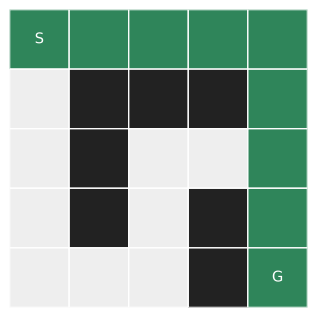
When the branching factor explodes and no cheap admissible heuristic exists, Monte Carlo tree search (MCTS) replaces exhaustive expansion with sampling: it selects a promising child by a score that balances value and exploration, \mathrm{UCB}(i) = \bar X_i + c\sqrt{\ln N / n_i}, expands one action, estimates value by rollout or a learned evaluator, and backpropagates. Chapter 31 runs MCTS inside planning over a learned world model, where this bridge’s A* would be too rigid; Chapter 8 connects the same budgeted-search idea to test-time compute. Other formalisms trade flexibility for crisper guarantees, and the value of each is what it can actually promise:
| Technique | Guarantee or property | Agent-system role |
|---|---|---|
| A* | optimal path with an admissible heuristic | route or tool-sequence search |
| MCTS | budgeted exploration guided by value estimates | planning in large branching spaces |
| SAT/SMT | a satisfying assignment or a proof of its absence | verify schedules, permissions, resource limits |
| PDDL/HTN | explicit preconditions, effects, decompositions | auditable workflow planning |
| behavior tree | reactive priority and fallback structure | bounded runtime control |
The 2026 pattern is hybrid, not replacement: models interpret and propose, search allocates computation, and formal or deterministic components check what they can genuinely guarantee.
A.6 Sequential decisions and reinforcement-learning vocabulary
A Markov decision process (MDP) is a tuple (\mathcal S, \mathcal A, P, R, \gamma): states, actions, a transition distribution, a reward, and a discount \gamma \in [0, 1). The agent observes s_t, acts, is rewarded, and transitions; it seeks a policy maximizing the discounted return G_t = \sum_{k\ge 0} \gamma^k r_{t+k+1}. The Markov assumption — that the current state holds everything from history needed to predict what comes next — is what makes the problem tractable, and Figure A.6 shows what happens when it fails: a partially observable MDP (POMDP) separates latent state s_t from observation o_t, and the agent must act on a belief, a distribution over latent states given history.
flowchart LR
    subgraph MDP
      S1["state s_t"] --> ACT1["action"]
      ACT1 --> S2["state s_t+1"]
    end
    subgraph POMDP
      L["latent state s_t"] -->|emits| O["observation o_t"]
      O --> B["belief / context"]
      B --> ACT2["action"]
    end
This picture is the RL section’s real payload for the book: an LLM agent’s context is a belief proxy, not a state. It holds selected messages, tool results, summaries, and retrieved memory — never the environment itself — so “the model saw it earlier” is not a state invariant, and compaction, retrieval, and observation freshness decide what the controller actually believes. To make “MDP” more than a tuple, we run value iteration on a three-state chain where only the goal pays.
# @save
def value_iteration(sweeps: int, gamma: float = 0.9) -> list[list[float]]:
    """Return the value estimate after each sweep on a three-state reward chain.

    A minimal MDP: states 0 and 1 move deterministically toward an absorbing
    goal state 2 that pays one unit. Each Bellman backup sets a state's value to
    its reward plus the discounted value of its successor, so the goal's reward
    propagates one step backward per sweep — the mechanism behind every dynamic
    program in RL, shown at a scale you can check by hand.

    Args:
        sweeps: Number of full backups to perform.
        gamma: Discount factor in [0, 1).

    Returns:
        The list of value vectors, one per sweep.
    """

    reward = {0: 0.0, 1: 0.0, 2: 1.0}
    values = {0: 0.0, 1: 0.0, 2: 0.0}
    history = []
    for _ in range(sweeps):
        updated = dict(values)
        for s in (0, 1, 2):
            updated[s] = reward[s] + (0.0 if s == 2 else gamma * values[s + 1])
        values = updated
        history.append([round(values[s], 3) for s in (0, 1, 2)])
    return history
for i, row in enumerate(value_iteration(3), start=1):
print(f"sweep {i}: V = {row}")sweep 1: V = [0.0, 0.0, 1.0]
sweep 2: V = [0.0, 0.9, 1.0]
sweep 3: V = [0.81, 0.9, 1.0]The reward at the goal walks backward one state per sweep — 1.0, then 0.9 at its neighbor, then 0.81 two steps out — which is discounting made visible. Now the clarifying question, priced this time in bits rather than utility. An agent is unsure whether a user wants a refund or a replacement (a fifty-fifty prior, one bit of uncertainty). It can ask “do you want your money back?”, which a refund-seeker answers yes to ninety percent of the time and a replacement-seeker only twenty percent. The information gain is the prior entropy minus the expected posterior entropy — the mutual information between the answer and the hidden intent.
# @save
def clarifying_info_gain(prior_a: float, p_yes_given_a: float, p_yes_given_b: float) -> dict[str, float]:
    """Return the expected information gain, in bits, of a clarifying question.

    Models a binary latent intent and a binary answer. Computes the prior
    entropy, the belief after each possible answer, and the entropy remaining on
    average; the reduction is the mutual information between question and intent
    — the information-theoretic value of asking, complementary to the utility
    VOI of the decision-theory section.

    Args:
        prior_a: Prior probability of the first intent.
        p_yes_given_a: P(answer yes | first intent).
        p_yes_given_b: P(answer yes | second intent).

    Returns:
        A dict with P(yes), the two posteriors on the first intent, and the gain.
    """

    def h(p: float) -> float:
        return 0.0 if p in (0.0, 1.0) else -(p * math.log2(p) + (1 - p) * math.log2(1 - p))

    p_yes = prior_a * p_yes_given_a + (1 - prior_a) * p_yes_given_b
    post_yes = prior_a * p_yes_given_a / p_yes
    post_no = prior_a * (1 - p_yes_given_a) / (1 - p_yes)
    expected_post = p_yes * h(post_yes) + (1 - p_yes) * h(post_no)
    return {
        "p_yes": p_yes,
        "posterior_if_yes": post_yes,
        "posterior_if_no": post_no,
        "info_gain_bits": h(prior_a) - expected_post,
    }
for name, value in clarifying_info_gain(0.5, 0.9, 0.2).items():
print(f"{name:18s} {value:.3f}")p_yes 0.550
posterior_if_yes 0.818
posterior_if_no 0.111
info_gain_bits 0.397The question buys about 0.40 bits — it does not fully resolve the intent (a “yes” leaves an eighteen-percent chance of replacement) but it moves the belief enough to change the next action, which is the sequential version of the VOI test. The last piece of vocabulary is exploration. A bandit is an MDP with one state: pull an arm, see a reward, learn. Cumulative regret measures the gap to always pulling the best arm, and the point of a bandit demo is that greedily exploiting your current estimate can lock onto the wrong arm forever.
# @save
def bandit_regret(strategy: str, seed: int, rounds: int = 300) -> float:
    """Return cumulative regret for a two-armed bandit under a given strategy.

    Two arms pay off with fixed probabilities; the better arm is unknown. The
    ``ucb`` strategy adds an exploration bonus that shrinks as an arm is pulled,
    so it keeps sampling the uncertain arm; the ``greedy`` strategy commits to
    whichever arm looked best after one pull each and can lock onto the loser.
    Regret is the reward given up versus always pulling the best arm.

    Args:
        strategy: Either ``"ucb"`` or ``"greedy"``.
        seed: Seed for the deterministic reward stream.
        rounds: Number of pulls.

    Returns:
        Total regret accumulated over all rounds.
    """

    rng = random.Random(seed)
    means = [0.3, 0.6]
    counts, sums, regret = [0, 0], [0.0, 0.0], 0.0
    for t in range(1, rounds + 1):
        if min(counts) == 0:
            arm = counts.index(0)
        elif strategy == "ucb":
            scores = [sums[i] / counts[i] + math.sqrt(2 * math.log(t) / counts[i]) for i in (0, 1)]
            arm = scores.index(max(scores))
        else:
            arm = 0 if sums[0] / counts[0] >= sums[1] / counts[1] else 1
        reward = 1.0 if rng.random() < means[arm] else 0.0
        counts[arm] += 1
        sums[arm] += reward
        regret += max(means) - means[arm]
return regretprint(f"UCB regret = {bandit_regret('ucb', 1):.1f}")
print(f"greedy regret = {bandit_regret('greedy', 1):.1f}")UCB regret = 7.8
greedy regret = 89.7The greedy strategy accumulates roughly ten times the regret, because an unlucky early sample on the good arm sends it to the bad arm and it never looks back. Online prompt or model selection can resemble a contextual bandit, but only once interference, delayed effects, and policy constraints are handled. RL is the study of sequential decisions under feedback, not a synonym for one gradient estimator; its variants — offline, inverse, constrained, and hierarchical RL — are named in Chapter 23, which supplies the route-appropriate training machinery this bridge deliberately does not derive.
A.7 A control-theory lens on agent loops
Control theory asks how a controller drives a system toward a target using observations and actions, and it maps onto an agent loop term for term.
| Control term | Agent-system counterpart |
|---|---|
| setpoint / reference | goal, target state, or SLO |
| controller | model plus deterministic harness |
| plant | external software or physical environment |
| actuator | tool or action interface |
| sensor | observation, tool result, telemetry |
| disturbance | user change, outage, adversary, noise |
An open-loop controller acts without measuring the result — a fixed generated plan executed to the end. A closed-loop controller observes outcomes and corrects, but it is only genuinely closed-loop when observations are timely, relevant, and actually change the action. Figure A.7 locates which box owns correction.
flowchart LR
    GOAL["Goal / setpoint"] --> ERROR(("compare"))
    OBS["Observed state"] --> ERROR
    ERROR --> CTRL["Controller<br/>model + harness"]
    CTRL -->|"bounded action"| TOOL["Tool / actuator"]
    TOOL --> ENV["Environment / plant"]
    DIST["Disturbance"] --> ENV
    ENV -->|"sensor + delay"| OBS
Feedback with lag can destabilize, and this is not abstract for agents: a worker retries because a write is not yet visible, both writes land, and now it compensates twice. We simulate the error dynamics of a proportional controller correcting on an observation that is d steps stale, e_{t+1} = e_t - K\,e_{t-d}, across three gain-and-delay settings.
# @save
def error_dynamics(gain: float, delay: int, steps: int = 40, start: float = 1.0) -> list[float]:
    """Return the error trajectory of a proportional controller with lag.

    Each step corrects the error using a correction proportional to a possibly
    stale observation of it, e[t+1] = e[t] - gain * e[t-delay]. With no delay
    and moderate gain the error decays; add delay, or push the gain up, and the
    correction fights yesterday's error, producing sustained or growing
    oscillation — the control-theoretic shape of a retry storm.

    Args:
        gain: Proportional correction strength K.
        delay: Observation staleness in steps.
        steps: Number of steps to simulate.
        start: Initial error.

    Returns:
        The error at each step, starting from ``start``.
    """

    history = [start]
    for t in range(steps):
        observed = history[t - delay] if t - delay >= 0 else start
        history.append(history[-1] - gain * observed)
    return history
for gain, delay in ((0.5, 0), (1.0, 1), (1.3, 1)):
trace = error_dynamics(gain, delay)
sample = [round(trace[i], 2) for i in (0, 5, 10, 20, 40)]
print(f"K={gain} delay={delay}: e at t=0,5,10,20,40 -> {sample}")K=0.5 delay=0: e at t=0,5,10,20,40 -> [1.0, 0.03, 0.0, 0.0, 0.0]
K=1.0 delay=1: e at t=0,5,10,20,40 -> [1.0, 1.0, 0.0, -1.0, 0.0]
K=1.3 delay=1: e at t=0,5,10,20,40 -> [1.0, 2.44, 3.49, -9.33, 51.87]The three regimes are exactly the ones an operator sees. With no lag and a gain of 0.5 the error decays to zero; add one step of delay at unit gain and it oscillates forever without settling; push the gain to 1.3 and the oscillation grows, diverging past fifty within forty steps. Figure A.8 plots all three. The fixes are the deadband and hysteresis: a deadband ignores small errors near the target, and hysteresis uses a higher threshold to enter a state than to leave it, so a circuit breaker opens on a spike but closes only after a sustained recovery, preventing the flap. Agent stop conditions, escalation, autoscaling, and circuit breakers all want this. The review questions are the control-theoretic ones: is the system observable — can we tell from outputs whether the external effect committed? — and controllable — can our tools reach a safe reconciled state? If either answer is no, better prompting will not repair the interface.
Show the code that draws this figure
import matplotlib.pyplot as plt

fig, ax = plt.subplots(figsize=(6.4, 3.2))
for gain, delay, label in ((0.5, 0, "K=0.5, no lag (stable)"),
                           (1.0, 1, "K=1.0, lag 1 (oscillates)"),
                           (1.3, 1, "K=1.3, lag 1 (diverges)")):
    ax.plot(error_dynamics(gain, delay), label=label)
ax.axhline(0, color="0.6", lw=0.8)
ax.set_ylim(-12, 12)
ax.set_xlabel("step")
ax.set_ylabel("error")
ax.legend(fontsize=8)
ax.spines[["top", "right"]].set_visible(False)
fig.tight_layout()
plt.show()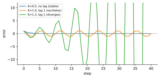
A.8 Distributed systems: partial failure, idempotency, and backpressure
Distributed components do not fail as one unit. A caller times out while a server keeps working; an acknowledgement is lost after an effect; a process restarts while another still holds state. This is partial failure, and its most dangerous shape is the ambiguous window: a worker sends an effect, the provider performs it, the response or the local commit is lost, and the worker cannot tell whether a retry duplicates the effect or a skip loses it. Delivery semantics do not make the effect atomic — at-most-once may lose work, at-least-once may duplicate it, and “exactly once” is only meaningful as an end-to-end property built from stable intent identity, atomic local state, and provider idempotency or reconciliation.
An idempotent operation produces the same external result when repeated with the same intent, so the key must identify the intent, not the delivery attempt — a fresh UUID per retry defeats deduplication. We build the smallest worker that makes this window executable, and break it twice. First the pieces: a task whose key hashes its intent, a provider that counts calls and effects, and a ledger that records intent status.
# @save
class InjectedCrash(RuntimeError):
    """Raised once, after an external effect and before the local commit."""


@dataclass(frozen=True)
class Task:
    """A notification intent carried by an at-least-once queue."""

    payment_id: str
    recipient: str

    @property
    def key(self) -> str:
        """Return an idempotency key derived from intent, not delivery attempt.

        Hashing the canonical intent fields means every redelivery of the same
        notification shares a key, so deduplication can recognize it; a key tied
        to the delivery instead would make each retry look like new work.
        """

        payload = json.dumps(
            {"payment_id": self.payment_id, "recipient": self.recipient}, sort_keys=True
        )
        return hashlib.sha256(payload.encode()).hexdigest()
The provider is the external world. It counts every call, and optionally honors the caller’s key so that a repeated call performs at most one effect — the behavior a real idempotent API offers.
# @save
class CountingProvider:
    """An external effect that counts calls and, optionally, deduplicates them."""

    def __init__(self, deduplicate: bool = False) -> None:
        self.deduplicate = deduplicate
        self.calls = 0
        self.effects = 0
        self.seen: set[str] = set()

    def send(self, task: Task) -> None:
        """Record one call and one externally visible effect, unless deduplicating."""

        self.calls += 1
        if self.deduplicate and task.key in self.seen:
            return
        self.seen.add(task.key)
        self.effects += 1
The ledger is the worker’s own memory of what it has started and finished. Reserving a key marks it pending; committing marks it done; an already-committed key refuses re-reservation. We keep it in SQLite to make the point that this is a real check-then-write, not a Python set.
# @save
class Ledger:
    """A local record of pending and committed intent keys.

    The reserve-then-commit shape is the crux of the lab: an intent becomes
    pending before the effect and committed only after, so a crash between the
    two leaves a pending row that cannot, by itself, say whether the external
    effect happened.
    """

    def __init__(self) -> None:
        self.connection = sqlite3.connect(":memory:")
        self.connection.execute("CREATE TABLE effects (key TEXT PRIMARY KEY, status TEXT NOT NULL)")

    def status(self, key: str) -> str | None:
        """Return the recorded status for an intent key, or None if unseen."""

        row = self.connection.execute("SELECT status FROM effects WHERE key = ?", (key,)).fetchone()
        return None if row is None else str(row[0])

    def reserve(self, key: str) -> bool:
        """Claim an intent as pending; refuse if it is already committed.

        Returns:
            True if the caller may proceed, False if the work is already done.
        """

        if self.status(key) == "committed":
            return False
        self.connection.execute(
            "INSERT OR IGNORE INTO effects(key, status) VALUES (?, 'pending')", (key,)
        )
        return True

    def commit(self, key: str) -> None:
        """Mark a reserved intent committed."""

        self.connection.execute("UPDATE effects SET status = 'committed' WHERE key = ?", (key,))
The worker ties them together: reserve, perform the effect, commit. Figure A.9 shows where a duplicate enters — the crash lands after the provider effect but before the commit, so the redelivered intent finds a pending row and cannot know the effect already happened.
sequenceDiagram
    participant Q as At-least-once queue
    participant W as Worker
    participant L as Local ledger
    participant P as External provider
    Q->>W: deliver intent, key=k
    W->>L: reserve k -> pending
    W->>P: perform effect, key=k
    P-->>W: effect completed
    Note over W: crash before local commit
    Q->>W: redeliver same intent, key=k
    W->>L: status(k) = pending
    Note over W,P: ambiguous: retry may duplicate, skip may lose
# @save
def fixture_deliveries(task_count: int = 20) -> list[Task]:
    """Return an at-least-once stream: unique tasks with a duplicate every fifth."""

    unique = [Task(f"payment-{i:02d}", f"user-{i:02d}@example.test") for i in range(task_count)]
    stream: list[Task] = []
    for i, task in enumerate(unique, start=1):
        stream.append(task)
        if i % 5 == 0:
            stream.append(task)
    return stream


def run_naive(deliveries: list[Task], provider: CountingProvider) -> None:
    """Execute every delivery with no ledger — the un-deduplicated baseline."""

    for task in deliveries:
        provider.send(task)


class IdempotentWorker:
    """Reserve, perform, then commit — exposing the effect-before-commit window."""

    def __init__(self, ledger: Ledger, provider: CountingProvider) -> None:
        self.ledger = ledger
        self.provider = provider
        self.crashed: set[str] = set()

    def process(self, task: Task, crash_after_effect_for: str | None = None) -> str:
        """Process one delivery, optionally crashing once in the ambiguous window.

        Reserves the intent, performs the external effect, and commits — but if
        asked, raises exactly once *after* the effect and *before* the commit,
        reproducing the partial failure that a local ledger alone cannot resolve.

        Args:
            task: The delivered intent.
            crash_after_effect_for: Payment id to crash on once, or None.

        Returns:
            ``"committed"`` for new work, ``"duplicate:committed"`` for a skip.
        """

        if not self.ledger.reserve(task.key):
            return "duplicate:committed"
        self.provider.send(task)
        if crash_after_effect_for == task.payment_id and task.key not in self.crashed:
            self.crashed.add(task.key)
            raise InjectedCrash(task.payment_id)
        self.ledger.commit(task.key)
        return "committed"

    def drain(self, deliveries: list[Task], crash_after_effect_for: str | None = None) -> int:
        """Drain the stream, retrying crashed intents, and return the crash count."""

        crashes, retry = 0, []
        for task in deliveries:
            try:
                self.process(task, crash_after_effect_for)
            except InjectedCrash:
                crashes += 1
                retry.append(task)
        for task in retry:
            self.process(task, crash_after_effect_for)
        return crashes


def build_report() -> dict[str, object]:
    """Run the four break-it drills and return their call and effect counts.

    Runs the same twenty-task, four-duplicate stream through the naive worker,
    the ledgered worker with no crash, the ledgered worker crashed once in the
    ambiguous window, and the crashed worker against a deduplicating provider.
    The counts are the lab's whole argument, so they are returned rather than
    printed.

    Returns:
        A nested dict of calls and effects for each of the four drills.
    """

    deliveries = fixture_deliveries()
    naive = CountingProvider()
    run_naive(deliveries, naive)

    local = CountingProvider()
    IdempotentWorker(Ledger(), local).drain(deliveries)

    ambiguous = CountingProvider()
    ambiguous_crashes = IdempotentWorker(Ledger(), ambiguous).drain(deliveries, "payment-07")

    dedup = CountingProvider(deduplicate=True)
    dedup_crashes = IdempotentWorker(Ledger(), dedup).drain(deliveries, "payment-07")

    return {
        "unique_tasks": 20,
        "deliveries": len(deliveries),
        "naive": {"calls": naive.calls, "effects": naive.effects},
        "local_ledger": {"calls": local.calls, "effects": local.effects},
        "ambiguous_window": {"crashes": ambiguous_crashes, "calls": ambiguous.calls, "effects": ambiguous.effects},
        "provider_key": {"crashes": dedup_crashes, "calls": dedup.calls, "effects": dedup.effects},
    }
Now we run all four drills and print their counts:
print(json.dumps(build_report(), indent=2)){
"unique_tasks": 20,
"deliveries": 24,
"naive": {
"calls": 24,
"effects": 24
},
"local_ledger": {
"calls": 20,
"effects": 20
},
"ambiguous_window": {
"crashes": 1,
"calls": 21,
"effects": 21
},
"provider_key": {
"crashes": 1,
"calls": 21,
"effects": 20
}
}The counts tell the whole story, and Table A.1 lays them side by side.
| Drill | Provider calls | External effects | Meaning |
|---|---|---|---|
| naive, no ledger | 24 | 24 | queue duplicates over-execute |
| local ledger, no crash | 20 | 20 | ordinary redelivery collapses cleanly |
| crash after effect | 21 | 21 | local state cannot resolve the ambiguous window |
| crash + provider key | 21 | 20 | repeated call, one effect: the window is closed at the provider |
The lesson is precise: a local ledger fixes ordinary duplicates but not the crash window, because the pending row is genuinely ambiguous — the fix has to live at the provider, as an idempotency key it deduplicates on, or as reconciliation. Multi-worker exclusion, key lifetime, transactional outbox, and saga compensation are Chapter 26’s job; this lab stops exactly at the point where one worker and one local ledger can go no further.
Capacity is the other half of distributed reasoning. Little’s law, L = \lambda W, relates the average number of items in a stable system to the arrival rate and the time each spends inside; with a fan-out a of downstream items per request it becomes L = \lambda a W.
lam, fan_out, residence = 20, 3, 2
print(f"in-flight downstream items = {lam} * {fan_out} * {residence} = {lam * fan_out * residence}")
in-flight downstream items = 20 * 3 * 2 = 120At twenty requests a second, fan-out three, and two seconds of downstream residence, expect about a hundred and twenty items in flight before any headroom. If the service rate ever falls below the arrival rate, there is no finite steady state and the queue grows without bound. Little’s law describes the state; it does not create capacity. The response is a bounded queue that produces backpressure — when it fills, callers wait, degrade, shed, or reject rather than consume unlimited memory — together with bounded retries, jittered backoff, honored retry-after signals, and one deadline budget shared across layers, because retries amplify load precisely when a dependency is already weak.
A.9 Threat modeling: assets, boundaries, and attack trees
Threat modeling is a design activity, not a penetration test or a launch-day form. A useful pass asks four questions: what are we building, what can go wrong, what will we do about it, and did we do a good job? It starts from assets — data, credentials, money, availability, model integrity, audit evidence, user trust, physical safety — and a data-flow diagram whose trust boundaries mark every place data or authority crosses between zones with different assumptions. Model input is a boundary crossing even when it arrives from an internal document, which is the whole reason indirect prompt injection is possible.
An attack tree starts from an adversary goal and decomposes it: OR children are alternative paths, AND children must all occur. Figure A.10 draws one for the naive retrieval agent Chapter 24 attacks, whose goal is an unauthorized disclosure or irreversible action. The tree exposes which control cuts which path — and, read against Chapter 24’s layered rebuild, why no single control suffices.
flowchart TD
    ROOT["OR: agent performs unauthorized disclosure or action"]
    ROOT --> DIRECT["Direct injection<br/>in the user turn"]
    ROOT --> INDIRECT["Indirect injection<br/>via retrieved document"]
    ROOT --> BYPASS["Bypass the action<br/>permission check"]
    DIRECT -.cut by.-> C1["Instruction/data separation"]
    INDIRECT -.cut by.-> C2["Quarantined reader + egress allowlist"]
    BYPASS -.cut by.-> C3["Policy enforcement point + bound approval"]
STRIDE — spoofing, tampering, repudiation, information disclosure, denial of service, elevation of privilege — is a checklist that improves coverage, but it is not the threat model; the model is the concrete assets, flows, assumptions, attacker goals, controls, tests, and residual risks of this system. The agent-specific extension is one sentence long: untrusted content can steer a probabilistic planner that holds tools, so separate instructions from data, minimize tool authority, validate typed proposals, and let deterministic code own the effects. Chapter 24 builds exactly that architecture and re-runs the attack suite against it.
A.10 Carrying the bridge forward
The durable move in each section outlasts any model release: condition belief on evidence, then combine it with loss; separate observation from intervention before trusting a comparison; keep hard constraints out of the blended score; use explicit search and solvers where their guarantees matter; treat an agent’s context as a belief, not a state; expect feedback lag to oscillate; design for partial failure and bound your queues; and threat-model every authority crossing. Each idea came with a number you ran, and each points at the chapter that spends it. When the book reorganizes, the consumption map at the top is what to update; the classical ideas and their design-review questions do not move.
A.11 Exercises
Using
value_of_signal, compute VOI for support-ticket triage under your own false-negative and false-positive losses. Find the observation cost at which asking becomes negative-value, and confirm it equals the printed VOI.Construct two forecasters where one has higher thresholded accuracy but a worse expected log loss. Using
log_lossandbrier, show the ranking flips, and argue which estimate you would let gate a release.In
simulate_routing, make the routing depend on difficulty even more strongly and re-runnaive_effectandbackdoor_effect. How large can the confounding grow before the naive estimate changes sign? Then name one variable that would be dangerous to add to the adjustment set, and why.Add latency as a third objective to
POINTS. Exhibit a weighted-sum winner that violates a hard latency cap, then apply constraint-first lexicographic selection and show it picks a different configuration.Change
GRIDto add a shorter path behind a wall, and re-runastarwith the Manhattan heuristic and withh = 0. Report the path length and the expansion counts for each, and explain the gap in terms of admissibility.Using
clarifying_info_gain, find a question whose two answer-likelihoods give high information gain but whose utility VOI is low (the resolved intent does not change the action). Explain why an agent should still not ask it.Enumerate every crash boundary in
IdempotentWorker.process. For each, state the ledger status, the possible provider state, and the safe next action. Add a crash injected before the provider call and predict the counts before running it.A provider promises idempotency, so a teammate proposes deleting both the caller key and the local ledger. Using the attack tree, walk a design review through key expiry, caller-generated duplicates, audit, and cross-worker races, and state what you would keep.