# @save
from __future__ import annotations

from collections import Counter
from dataclasses import dataclass, replace
from typing import Sequence

REFUND_CUES = ("refund", "money back", "reverse the payment", "reverse payment",
               "charge back", "chargeback", "reimburse")
TECH_CUES = ("crash", "error", "freez", "logged me out", "won't load",
             "does not load", "broken", "bug", "500")
STATUS_CUES = ("where", "tracking", "package", "parcel", "shipped", "arrive",
               "delivery", "delivered", "eta")
DEFAULT_PRECEDENCE = ("refund", "status", "technical")


@dataclass(frozen=True)
class Ticket:
    text: str
    expected: str


@dataclass(frozen=True)
class Demo:
    text: str
    label: str


@dataclass(frozen=True)
class Prompt:
    instruction: str
    precedence: tuple[str, ...] = DEFAULT_PRECEDENCE
    demos: tuple[Demo, ...] = ()


def _content_tokens(text: str) -> set[str]:
    return {w.strip(".,?!;:'\"-").lower() for w in text.split() if len(w) > 2}


def _similarity(a: str, b: str) -> float:
    ta, tb = _content_tokens(a), _content_tokens(b)
    return len(ta & tb) / min(len(ta), len(tb)) if ta and tb else 0.0


def _prior_label(text: str, precedence: tuple[str, ...]) -> str:
    lower = text.lower()
    hits = {
        "refund": any(cue in lower for cue in REFUND_CUES),
        "technical": any(cue in lower for cue in TECH_CUES),
        "status": any(cue in lower for cue in STATUS_CUES),
    }
    for label in precedence:
        if hits[label]:
            return label
    return "technical"


def _nearest_demo(text: str, demos: Sequence[Demo]) -> tuple[Demo | None, float]:
    best, best_sim = None, 0.0
    for demo in demos:
        sim = _similarity(text, demo.text)
        if sim > best_sim:
            best, best_sim = demo, sim
    return best, best_sim


def classify(prompt: Prompt, text: str, demo_threshold: float = 0.5) -> str:
    """Route one ticket with the stub proxy: nearest demonstration, else keyword prior.

    The stub imitates two real phenomena cheaply. When a demonstration is close
    enough it completes that demonstration's label (the in-context-learning
    path); otherwise it falls back to keyword cues resolved by a precedence
    order (its "prior" behavior). It is a keyword matcher, not a model: its job
    is to make every downstream score explainable, not to be good at English.

    Args:
        prompt: The prompt configuration — its precedence order and any
            demonstrations both steer the routing.
        text: The customer ticket to classify.
        demo_threshold: Minimum token-overlap similarity at which the nearest
            demonstration overrides the keyword prior.

    Returns:
        One of ``"refund"``, ``"status"``, or ``"technical"``.
    """
    if prompt.demos:
        demo, sim = _nearest_demo(text, prompt.demos)
        if demo is not None and sim >= demo_threshold:
            return demo.label
return _prior_label(text, prompt.precedence)13 Prompting and Context Engineering
On Friday afternoon a ticket router starts sending delivery complaints to the refunds queue. Its prompt changed that morning: one adjective, in a paragraph that has been edited dozens of times. The team can show the current prompt and the current failures. It cannot show which edit caused the regression, which cases improved, which model revision ran, or whether the context around the prompt also moved. Reverting the adjective rescues five hand-picked examples, so they ship the revert. Monday, a different slice fails. That is not a wording problem. It is an experimental-design problem, and this chapter treats it as one.
We build the context pipeline for that router and measure it at every step: (i) a scorer over a frozen case set that prints a failure table, not just a number; (ii) an automatic prompt optimizer whose candidates are generated from failure traces, with its development and held-out scores tracked round by round; (iii) a typed assembler that renders distributed application state into one ordered, trust-labelled input and refuses to silently drop the query; (iv) two context failures — distraction and confusion — reproduced live and then repaired; (v) a cache-aware prefix layout whose reusable-byte fraction we measure; and (vi) a survival-checked compactor driven across a 50-turn simulation whose utilization and prefix reuse we plot. Everything runs offline against a small deterministic stub classifier whose entire script is on the page. That stub is not a language model — its scores are evidence about the control flow around a model, never about a model’s language ability. Chapter 12 established the message and tool-call wire format this chapter fills; Chapter 22 builds the full evaluation program this chapter only samples.
13.1 Prompting is measurement before wordsmithing
A prompt is not a string. It is executable configuration applied to one model on one input distribution, and a useful record of it is a tuple
P=(m,v,i,d,s,c,g), \tag{13.1}
where m is the exact model revision, v the prompt version, i the instructions, d the demonstrations, s the output schema, c the decoding controls, and g the context-assembly policy. Its quality is defined only relative to an evaluation distribution D and a metric M:
Q(P)=\mathbb{E}_{x\sim D}\!\left[M(P,x)\right]. \tag{13.2}
Changing “precise” to “careful” changes P. So does adding a tool, moving a timestamp, reordering examples, or compacting history. If two variants are not run on the same versioned cases with the same scorer and model, the comparison is anecdote. That is the whole discipline, and everything below is an instance of it.
To measure anything offline we need something to measure. We use a deterministic stub: a proxy “classifier” whose behavior the reader can fully inspect, so that when a score moves we know exactly why. It routes a customer ticket to refund, status, or technical using keyword cues and a precedence order, and — this is the part that will matter for in-context learning — it will complete the label of the most similar demonstration when one is close enough. We start with just the keyword prior.
The scorer freezes a case set and, crucially, keeps the per-case failures. A single aggregate hides whether a rise from 82 to 86 percent fixed four hard cases or swapped eight. Exact match works here because the labels are finite; a rubric grader would work for an explanation, but then the grader, its calibration cases, and its disagreement rate all become part of the measurement system. No scorer is “just evaluation.”
# @save
DEV_SET = (
    Ticket("Where is order 41? The tracking page has not moved.", "status"),
    Ticket("The desktop app crashes on launch every time.", "technical"),
    Ticket("Please refund the duplicate charge on my card.", "refund"),
    Ticket("My package says delivered, but it is not here.", "status"),
    Ticket("The tracking page crashes whenever I open it.", "technical"),
    Ticket("I want my money back because the parcel is late.", "refund"),
    Ticket("Reset links always return a server error.", "technical"),
    Ticket("Has order 77 shipped yet?", "status"),
    Ticket("Cancel and refund the order that has not shipped.", "refund"),
    Ticket("The delivery screen freezes after sign-in.", "technical"),
    Ticket("You charged me twice for one order.", "refund"),
    Ticket("You charged me twice; refund one of the two order charges.", "refund"),
)

HELDOUT_SET = (
    Ticket("The checkout page throws an error at payment.", "technical"),
    Ticket("Where is my parcel? Tracking stopped three days ago.", "status"),
    Ticket("Refund me; the shipment never arrived.", "refund"),
    Ticket("The delivery map freezes and the app crashes.", "technical"),
    Ticket("Two identical payments left my account this week.", "refund"),
    Ticket("Please reimburse the charge for the broken item.", "refund"),
)

BASELINE = Prompt("Classify the customer ticket. Return one label.")


def evaluate(prompt: Prompt, examples: Sequence[Ticket]) -> dict:
    """Score a prompt on a case set and keep the per-case failure rows.

    Args:
        prompt: The prompt configuration to score.
        examples: The frozen cases to run it against.

    Returns:
        A dict with the exact-match ``score`` in ``[0, 1]``, the list of
        ``failures`` (each an expected/actual/text row), and every ``rows``
        prediction — the failure rows, not the scalar, are the primary artifact.
    """
    rows, failures = [], []
    for item in examples:
        actual = classify(prompt, item.text)
        row = {"text": item.text, "expected": item.expected, "actual": actual}
        rows.append(row)
        if actual != item.expected:
            failures.append(row)
    score = (len(examples) - len(failures)) / len(examples)
    return {"score": score, "failures": failures, "rows": rows}
Run the baseline and read its failures, not only its score.
base = evaluate(BASELINE, DEV_SET)
print(f"baseline dev score: {base['score']:.3f} "
      f"({len(DEV_SET) - len(base['failures'])}/{len(DEV_SET)})")
for f in base["failures"]:
    print(f"  expected {f['expected']:9} got {f['actual']:9} | {f['text']}")
baseline dev score: 0.750 (9/12)
expected technical got status | The tracking page crashes whenever I open it.
expected technical got status | The delivery screen freezes after sign-in.
expected refund got technical | You charged me twice for one order.Two of the three failures share a signature — a malfunction described with delivery vocabulary, routed to status because the default precedence checks status before technical. The third is different: a refund request with no refund cue word at all. A single aggregate would have told us “83 percent” and hidden that these are two distinct problems needing two distinct fixes. Prompting is measurement before it is wordsmithing, and the failure table is where the measurement starts.
13.2 In-context learning: examples are a dataset in the prompt
The third failure hints at the most important lever after the instruction: demonstrations. In-context learning changes behavior by conditioning the forward pass on examples in the prompt; it does not update the checkpoint’s weights (Brown et al. 2020). Mechanistically, the demonstrations are earlier positions in the same sequence, and the query at the end attends back over them: a query near a demonstrated input completes the pattern the demonstration set — its input-to-output mapping, its label vocabulary, its output shape. Figure 13.1 draws that path.
flowchart LR
    D1["demo: 'app crashes' -> technical"] --> Q
    D2["demo: 'where is my order' -> status"] --> Q
    D3["demo: 'refund the charge' -> refund"] --> Q
    Q["query: 'the billing page errors'"] --> A["attend to nearest demo pattern"]
    A --> O["complete its label: technical"]
That density is why examples are powerful and dangerous: a demonstration teaches format, label space, and a decision rule all at once, so a corrupted one teaches a corrupted rule. Min et al. (2022) found that on real models demonstrations mainly convey the label space, format, and input distribution, and that the effect of label correctness is model- and task-dependent (Min et al. 2022). Our stub takes the strong form for clarity: it copies the nearest demonstration’s label. We can watch a single flipped label flip a nearby query.
query = "The billing page throws an error when I submit the form."
clean = Prompt(BASELINE.instruction,
               demos=(Demo("The billing page shows an error on submit.", "technical"),))
poisoned = Prompt(BASELINE.instruction,
                  demos=(Demo("The billing page shows an error on submit.", "status"),))
print("clean demonstration    ->", classify(clean, query))
print("corrupted demonstration->", classify(poisoned, query))
clean demonstration -> technical
corrupted demonstration-> statusThe corrupted demonstration drags a technical ticket to status, and nothing about the instruction changed. Because examples are a small dataset embedded in the request, apply dataset discipline: choose cases near the ambiguity boundary rather than five easy duplicates; cover labels and high-cost failure modes; make the demonstrated output identical to the production schema; strip accidental features (a customer name, a formatting quirk) that should not control the answer; fix order while measuring and then test order sensitivity; and keep a held-out set that selection never sees. A static demonstration set is easy to version and maximizes prefix reuse; query-dependent selection may be more relevant but adds retrieval error, latency, and cache variation. Compare both on the same distribution — “dynamic” is not automatically better.
Personas deserve the same skepticism. “You are a world-class expert” may change tone or verbosity on a given model and task, but it is not a general capability multiplier: a 2024 study evaluated 162 personas across four model families and 2,410 factual questions and found no overall accuracy improvement (Zheng et al. 2024). A role earns its place when it establishes audience, vocabulary, or an interaction contract the metric can detect — not because a status adjective is assumed to confer expertise.
13.3 Structure controls parsing, and reasoning is a measured control
Long prose makes boundaries implicit; structural markup makes them explicit to people, to template code, and often to the model. Fencing separates instructions, evidence, and the query, and names the provenance of each block.
document = "Refund window is 30 days from delivery."
fenced = (f'<retrieved_document trust="external" source="policy-v4">\n'
          f'{document}\n</retrieved_document>\n'
          f'<task trust="developer">\nAnswer only from the document.\n</task>')
print(fenced)
<retrieved_document trust="external" source="policy-v4">
Refund window is 30 days from delivery.
</retrieved_document>
<task trust="developer">
Answer only from the document.
</task>Use names that carry semantics — <untrusted_search_result> says more than <data> — close every delimiter, and render through one tested function so a mismatch is a caught serialization bug, not a silent prompt corruption. But markup is not an authorization boundary. Text inside <untrusted_search_result> can still contain an instruction-shaped sentence, and a model can still follow it. Trust labels give the prompt and the audit log information to reason with; they do not make hostile text inert. Chapter 24 owns injection defense, isolation, and least privilege; here the invariant is only preserve provenance, and never imply that fencing equals security.
The system prompt should operate at the right altitude: purpose, non-negotiable behavior, decision policy, tool-use expectations, and output contract — not a giant flowchart encoded in prose, and not slogans too vague to test. Where several roles supply text, the harness enforces an instruction hierarchy — system above developer above user above tool output — as executable precedence, not as a hope that the model honors the ordering. Chapter 7 owns behavior-specification design; this chapter renders the selected version and keeps it stable.
Reasoning is another versioned request control, not a magic phrase. “Think step by step” helped some early models and tasks and is not a durable default; modern reasoning-tuned models expose a reasoning effort, thinking budget, or thinking level, and some return only a summary of hidden work. Treat the setting like any other knob: evaluate task success, latency, and input and output token usage, and pick the point that clears the bar. The tradeoff is real and monotone in cost, and it is worth a representative sketch before you commit engineering to it.
| Reasoning effort | Task success | Output tokens | Latency | When to pick it |
|---|---|---|---|---|
| low | adequate on easy cases | small | low | high-volume, shallow routing |
| medium | better on multi-step cases | moderate | moderate | most agent steps |
| high | best on the hardest cases | large | high | rare, high-value, checkable tasks |
The table is representative, not a recorded run — the numbers depend entirely on the model and task. The durable rule survives the numbers: do not require a hidden chain of thought as an application contract; ask instead for checkable work products — assumptions, calculations, citations, tests, a concise rationale — when the task needs them, and measure whether the extra effort pays.
13.4 Automatic prompt optimization: where candidates come from
Once prompts have versions and scores, optimization becomes black-box search: pick P^\* = \arg\max_{P\in\mathcal{P}} \hat Q_D(P) over a candidate set \mathcal{P} scored on development cases. If a human writes every candidate, that is just hand-tuning with a scoreboard. What makes optimization automatic is a generator that proposes candidates on its own — and, as we did in Section 13.1, the failure table is exactly the raw material it needs. Figure 13.2 distinguishes the two.
flowchart LR
    subgraph loop["automatic loop"]
        E["evaluate on dev split"] --> R["reflect on failure traces"]
        R --> G["generate candidates:<br/>instruction edits + bootstrapped demos"]
        G --> E
    end
    E --> B["keep best; report dev vs held-out"]
Our generator has two operators, both derived from the current failures. The first reads the confusion matrix and proposes an instruction edit — a precedence clause that promotes the label being lost over the label it loses to. The second bootstraps a demonstration: it finds a currently-correct dev case near a failure and adds it as a labelled example, so the stub’s pattern-completion path can carry the fix. This is the shape of real systems — MIPROv2 jointly proposes instructions and bootstraps few-shot demonstrations under a Bayesian search (Opsahl-Ong et al. 2024); GEPA reflects in natural language over whole trajectories and keeps a Pareto frontier of candidates (Agrawal et al. 2025); DSPy packages both behind a compile step (Khattab et al. 2024) — reduced here to something small enough to read.
# @save
def _propose_precedence(current: tuple[str, ...], failures: Sequence[dict]) -> tuple[str, ...]:
    """Promote the most-confused expected label above the label it loses to."""
    confusion = Counter((f["actual"], f["expected"]) for f in failures)
    if not confusion:
        return current
    (lost_to, should_be), _ = confusion.most_common(1)[0]
    order = list(current)
    if lost_to in order and should_be in order and order.index(should_be) > order.index(lost_to):
        order.remove(should_be)
        order.insert(order.index(lost_to), should_be)
    return tuple(order)


def _bootstrap_demo(prompt: Prompt, dev: Sequence[Ticket], failures: Sequence[dict]) -> Demo | None:
    """Turn a currently-correct dev case near the first failure into a demonstration."""
    if not failures:
        return None
    fail = failures[0]
    existing = {d.text for d in prompt.demos}
    best, best_sim = None, 0.0
    for item in dev:
        if item.text in existing or item.text == fail["text"]:
            continue
        if item.expected != fail["expected"] or classify(prompt, item.text) != item.expected:
            continue
        sim = _similarity(fail["text"], item.text)
        if sim > best_sim:
            best, best_sim = item, sim
    return Demo(best.text, best.expected) if best is not None and best_sim >= 0.5 else None


def optimize_prompt(dev: Sequence[Ticket], heldout: Sequence[Ticket], rounds: int = 3) -> dict:
    """Search prompt space with a propose -> evaluate -> keep-best loop over a metric.

    Each round generates candidates from the current best prompt's failures — an
    instruction precedence edit and a bootstrapped demonstration — scores them
    all on ``dev``, and keeps the highest (ties break toward the earlier, simpler
    candidate). The held-out score is recorded but never optimized against, so a
    growing dev-minus-held-out gap exposes overfitting to the dev set.

    Args:
        dev: The development split the search is allowed to see.
        heldout: An untouched split, scored only for reporting.
        rounds: How many propose/evaluate rounds to run.

    Returns:
        A dict with the ``winner`` prompt and the per-round ``trajectory`` of
        dev and held-out scores.
    """
    best, trajectory = BASELINE, []
    for step in range(rounds + 1):
        dev_result = evaluate(best, dev)
        trajectory.append({
            "round": step,
            "dev_score": dev_result["score"],
            "heldout_score": evaluate(best, heldout)["score"],
            "n_demos": len(best.demos),
            "precedence": best.precedence,
        })
        if step == rounds:
            break
        candidates = []
        new_prec = _propose_precedence(best.precedence, dev_result["failures"])
        if new_prec != best.precedence:
            edited = best.instruction + f" PRECEDENCE: {' > '.join(new_prec)}."
            candidates.append(replace(best, instruction=edited, precedence=new_prec))
        demo = _bootstrap_demo(best, dev, dev_result["failures"])
        if demo is not None:
            candidates.append(replace(best, demos=best.demos + (demo,)))
        scored = [(evaluate(c, dev)["score"], -i, c) for i, c in enumerate(candidates)]
        scored.append((dev_result["score"], 1, best))
        best = max(scored, key=lambda t: (t[0], t[1]))[2]
    return {"winner": best, "trajectory": trajectory}
Run the loop and print the trajectory — the sequence of best scores, which is what tells us whether the search is learning or thrashing.
opt = optimize_prompt(DEV_SET, HELDOUT_SET)
for row in opt["trajectory"]:
    print(f"round {row['round']}: dev={row['dev_score']:.3f}  "
          f"held-out={row['heldout_score']:.3f}  demos={row['n_demos']}  "
          f"precedence={row['precedence']}")
winner = opt["winner"]
print("\nwinner instruction:", repr(winner.instruction))
print("winner demonstrations:", len(winner.demos))
round 0: dev=0.750 held-out=0.667 demos=0 precedence=('refund', 'status', 'technical')
round 1: dev=0.917 held-out=0.833 demos=0 precedence=('refund', 'technical', 'status')
round 2: dev=1.000 held-out=0.833 demos=1 precedence=('refund', 'technical', 'status')
round 3: dev=1.000 held-out=0.833 demos=1 precedence=('refund', 'technical', 'status')
winner instruction: 'Classify the customer ticket. Return one label. PRECEDENCE: refund > technical > status.'
winner demonstrations: 1Round 1 proposes the precedence edit from the two status/technical confusions and fixes them; round 2 bootstraps a demonstration for the cue-less refund case and reaches 12/12 on dev. Figure 13.3 plots both splits.
Show the code that draws this figure
import matplotlib.pyplot as plt

traj = opt["trajectory"]
rounds = [r["round"] for r in traj]
fig, ax = plt.subplots(figsize=(6.4, 3.3))
ax.plot(rounds, [r["dev_score"] for r in traj], marker="o", label="dev (searched)")
ax.plot(rounds, [r["heldout_score"] for r in traj], marker="s", ls="--",
        label="held-out (untouched)")
ax.set_xlabel("optimization round")
ax.set_ylabel("exact-match score")
ax.set_ylim(0.5, 1.05)
ax.set_xticks(rounds)
ax.legend()
fig.tight_layout()
plt.show()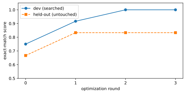
The gap is the lesson. Dev reaches 100 percent while the held-out set stops at 5/6 — the precedence edit generalizes (it fixes the held-out technical/status confusion too), but the bootstrapped demonstration is tuned to one dev case and does not carry to a held-out refund phrased differently. Optimization overfits prompts exactly as training overfits weights: searching more candidates against the same twelve cases leaks those cases into the winner. Keep a final set untouched, slice results by risk category, and re-test after model changes. An optimizer without a trustworthy metric accelerates the wrong behavior — verbosity that flatters a judge, demonstrations copied from the test set, loopholes in a unit test. Automatic optimization does not remove specification work; it makes specification quality more consequential.
NoteIn the interview
Q. Your optimizer lifted dev accuracy from 75% to 100%. Do you ship it? Not on that number. The searched split is contaminated by the search; the honest estimate is the untouched held-out split, which here sits at 83%, and the gap is overfitting, not progress. The trap is quoting the optimized metric as if it were a generalization estimate. Ship on held-out performance sliced by risk category, with a promotion gate defined before the search and a re-test after any model change.
13.5 Context is a constructed input, not a transcript
Prompt engineering asks “what instruction should I write?” Context engineering asks the larger question: what should the model see on this call? For an agentic application the context is a function
C_t=f(S,T,M,R,H_t,Q_t;B), \tag{13.3}
where S is the system instruction, T the tool descriptions, M durable remembered state, R retrieved evidence, H_t selected history, Q_t the current query, and B the token budget. The semicolon matters: the budget constrains the function, it is not another thing to concatenate. The window resembles RAM only in being finite working state; unlike RAM, its addresses are not equally reliable and an irrelevant resident token is not harmless. Chapter 3 separated admitted context from effective context — “Lost in the Middle” found position sensitivity on multi-document QA (Liu et al. 2024), and Chroma’s context-rot experiments found performance often degrading as input grows even under controlled constructions (Chroma Research 2025). Neither gives a safe percentage; together they retire “send everything because it fits.” The objective is the smallest high-signal input that makes the target behavior likely.
An assembler chooses, labels, orders, and budgets that state before the call. Figure 13.4 marks the boundary — and the ownership lines: Chapter 18 owns how M is represented, Chapters 14 and 15 own the quality of R, Chapter 17 owns T; this chapter consumes their outputs as typed segments and decides what enters the next call.
flowchart LR
    S["system contract"] --> A["deterministic assembler"]
    T["tool descriptions"] --> A
    M["durable state refs"] --> A
    R["retrieved evidence"] --> A
    H["selected history"] --> A
    Q["current query"] --> A
    B["token budget"] -. constrains .-> A
    A --> O["ordered, trust-labelled input"]
    O --> L["context ledger"]
Think in segments, not one growing string. Each carries at least a kind, a trust label, content, a stability flag, and a priority; a regulated system adds tenant, expiry, sensitivity, provenance, and a pointer to the source. The renderer sorts by a fixed table (stable to volatile), wraps each block with its kind and trust, and applies the budget at segment boundaries. A required system or query segment raises rather than disappears; lower-priority optional segments may be dropped, but selection should decide that before rendering so the reason is visible.
# @save
def token_count(text: str) -> int:
    return len(text.split())


@dataclass(frozen=True)
class Segment:
    """One typed unit of context with the metadata a policy can act on.

    ``kind`` fixes structural position; ``trust`` records who controls the
    content (provenance, not authorization); ``stable`` marks material that can
    form a reusable prefix; ``priority`` and ``tags`` drive selection.
    """

    kind: str
    trust: str
    content: str
    stable: bool = False
    priority: int = 0
    tags: tuple[str, ...] = ()


ORDER = {"system": 0, "tools": 1, "examples": 2, "retrieved": 3, "history": 4, "query": 5}


def render_context(segments: Sequence[Segment], budget: int) -> str:
    """Render typed segments into one deterministic, trust-labelled sequence.

    Segments are ordered stable-to-volatile by a fixed table, each wrapped with
    its kind and trust. The budget is applied at block boundaries: an optional
    over-budget segment is dropped, but a required system or query segment that
    will not fit raises instead of vanishing, so truncation can never silently
    delete policy or the user's question.

    Args:
        segments: The typed segments to assemble, in any order.
        budget: The whitespace-token proxy budget for the whole input.

    Returns:
        The assembled context string.

    Raises:
        ValueError: If a required (stable or query) segment exceeds the budget.
    """
    ordered = sorted(enumerate(segments), key=lambda pair: (ORDER[pair[1].kind], pair[0]))
    rendered, used = [], 0
    for _, segment in ordered:
        block = f'<{segment.kind} trust="{segment.trust}">\n{segment.content}\n</{segment.kind}>'
        size = token_count(block)
        if used + size > budget and not segment.stable and segment.kind != "query":
            continue
        if used + size > budget:
            raise ValueError(f"required {segment.kind} segment exceeds the {budget}-token budget")
        rendered.append(block)
        used += size
    return "\n".join(rendered)


def select_context(segments: Sequence[Segment], query: str) -> list[Segment]:
    """Keep stable segments, the query, high-priority items, and tag matches."""
    terms = _content_tokens(query)
    return [s for s in segments
            if s.stable or s.kind == "query" or s.priority >= 8 or terms & set(s.tags)]
Render a small window and read the assembled bytes — stable system first, evidence next, the query last, each labelled.
segments = [
    Segment("query", "user", "Where is order 41?"),
    Segment("system", "developer", "Route tickets by policy v4.", stable=True),
    Segment("retrieved", "tool", "order 41 shipped 2026-07-18", tags=("order",), priority=8),
]
print(render_context(segments, budget=40))
<system trust="developer">
Route tickets by policy v4.
</system>
<retrieved trust="tool">
order 41 shipped 2026-07-18
</retrieved>
<query trust="user">
Where is order 41?
</query>Silent truncation is the failure to design out. Dropping the end may delete the query; dropping the front may delete policy; cutting a serialized tool schema in half leaves invalid structure. So we budget at boundaries and fail closed when required material will not fit.
try:
    render_context([Segment("query", "user", "one two three four five six")], budget=3)
except ValueError as exc:
    print("raised:", exc)
raised: required query segment exceeds the 3-token budgetProduction budgeting uses the exact tokenizer and chat template from Chapter 12; the lab’s whitespace token_count is deliberately transparent and portable, and its counts must never be transferred to a hosted endpoint. Reconcile local rendered tokens against provider usage and alert on persistent drift — a hidden template or tool-description change is often eating the difference.
13.6 Four moves and the context-failure taxonomy
Four operations cover most caller-side context work, and naming them separately makes them easier to reason about. Write moves a durable fact outside the active window and leaves an addressable reference — not “remember everything,” just a compact pointer like REF incident-91: replay bundle and trace index, carrying enough scent (a name, a type, a one-line summary) to know when it matters. Select chooses the subset relevant to this decision, filtering by task, provenance, freshness, and permissions, not lexical overlap alone. Compress replaces detail with a smaller representation that preserves declared invariants. Isolate runs a noisy subtask in a separate context and returns only a digest. Figure 13.5 routes information to the right move.
flowchart TB
    X["candidate information"] --> D{"needed on this call?"}
    D -- "no, but durable" --> W["write externally, keep a reference"]
    D -- "yes, only a subset" --> S["select relevant segments"]
    D -- "yes, but too large" --> C["compress under survival invariants"]
    D -- "needs noisy independent work" --> I["isolate, return a digest"]
    W --> A["active context"]
    S --> A
    C --> A
    I --> A
These moves respond to four recurring content failures. The taxonomy organizes debugging; the labels are not mutually exclusive, and a stale summary can trigger several at once.
| Failure | What happens | First diagnostic | Typical response |
|---|---|---|---|
| poisoning | an early mistaken fact or plan persists and shapes later turns | trace its first appearance and every derived decision | replace or quarantine it; keep the correction and rationale |
| distraction | irrelevant detail crowds the window and changes behavior | remove one context class at a time | select fewer, higher-signal segments |
| confusion | similar tools, examples, or facts create an ambiguous choice | inspect competing names, descriptions, demonstrations | simplify, rename, or isolate the alternatives |
| clash | instructions or facts conflict with no precedence rule | render the full ordered context with provenance | resolve in application policy; do not ask the model to guess authority |
We saw poisoning in Section 13.2: a corrupted demonstration flipped a nearby query and persisted. Two more are reproducible with the machinery already built. Distraction first: preload six irrelevant promotional segments alongside one high-signal shipping fact under a tight budget, and the fact is crowded out of what the model would see. Selecting before rendering keeps it.
signal = Segment("retrieved", "tool", "order 41 shipped on 2026-07-18 via courier",
                 tags=("order",), priority=8)
distractors = [Segment("retrieved", "promo", f"promo note {i}") for i in range(6)]
query = Segment("query", "user", "Where is order 41?")
system = Segment("system", "developer", "Route by policy.", stable=True)
everything = [system, *distractors, signal, query]

preloaded = render_context(everything, budget=49)
selected = render_context(select_context(everything, "Where is order 41?"), budget=49)
print("preload  — shipping fact present:", "order 41 shipped" in preloaded)
print("selected — shipping fact present:", "order 41 shipped" in selected)
preload — shipping fact present: False
selected — shipping fact present: TrueThe high-signal fact is absent from the preloaded context and present after selection — the fix the taxonomy prescribes for distraction is exactly “select fewer, higher-signal segments.” Confusion next: two demonstrations that look alike but carry different labels leave the nearest-match rule an ambiguous choice, and it takes the wrong one; removing the conflicting demonstration restores the prior.
ambiguous = "Where is order 41? It still has not arrived."
confused = Prompt(BASELINE.instruction,
                  demos=(Demo("Order 41: refund it, it has not arrived.", "refund"),))
print("with a similar wrong-label demo:", classify(confused, ambiguous), "(expected status)")
print("with the demo removed:          ", classify(BASELINE, ambiguous))
with a similar wrong-label demo: refund (expected status)
with the demo removed: statusTwo failures, reproduced and repaired without a single API call, because the control flow — not the model — produced them. Isolation, the fourth move, is worth its own caution: it reduces distraction and protects the primary prefix, but it also loses tacit context and can hide errors behind a tidy summary, so require a return contract — conclusion, evidence, uncertainty, artifacts, open questions. Chapter 20 owns subagent topology; here we only define the boundary.
13.7 Prefix stability is a caller-side invariant
Chapter 10 established the serving mechanism: a prefix cache reuses previously computed key-value state only for an exact, compatible token prefix. Semantic similarity is irrelevant — a reordered schema, one whitespace-sensitive token, or a timestamp near the front ends reuse at the first differing byte. Caller-side layout decides whether such a prefix exists. Put slow-changing content first and fast-changing content last:
\underbrace{S\,\Vert\,T\,\Vert\,E}_{\text{stable prefix}}\ \Vert\ \underbrace{R_t\,\Vert\,H_t\,\Vert\,Q_t}_{\text{volatile suffix}}, \tag{13.4}
with S the system policy, T stable tool and schema material, and E fixed examples. Do not insert the current time, a request id, a user name, or a per-request feature flag before the stable prefix. We measure the break point directly: the reuse ends at the first differing byte.
# @save
def common_prefix_bytes(left: str, right: str) -> int:
    """Count identical leading bytes of two strings; the first difference ends reuse.

    A prefix cache can reuse KV state only up to the first byte at which two
    requests diverge, so this count is the caller-side diagnostic for how much
    of a request a stable layout keeps reusable.

    Args:
        left: The previous request's assembled bytes.
        right: The current request's assembled bytes.

    Returns:
        The number of identical leading UTF-8 bytes.
    """
    a, b = left.encode("utf-8"), right.encode("utf-8")
    for index, (one, two) in enumerate(zip(a, b)):
        if one != two:
            return index
    return min(len(a), len(b))


def cache_cost(stable_tokens: int, volatile_tokens: int, read_rate: float = 0.10) -> dict:
    """Illustrative cache economics: a hit reads the stable prefix at a discount."""
    hit = stable_tokens * read_rate + volatile_tokens
    miss = stable_tokens + volatile_tokens
return {"hit": hit, "miss": miss, "multiplier": miss / hit}print("stable layout, reuse ends at byte:",
common_prefix_bytes("STATIC-PREFIX\nA", "STATIC-PREFIX\nB"))
print("timestamp first, reuse ends at byte:",
common_prefix_bytes("NOW=11\nSTATIC-PREFIX", "NOW=12\nSTATIC-PREFIX"))stable layout, reuse ends at byte: 14
timestamp first, reuse ends at byte: 5A stable layout keeps the whole leading block reusable and breaks only where the turn genuinely differs; a timestamp at the front breaks reuse almost immediately. Figure 13.6 shows both cases as aligned token streams.
Show the code that draws this figure
from matplotlib.patches import Rectangle

fig, axes = plt.subplots(2, 1, figsize=(6.8, 3.2))
prev_stable = ["SYSTEM", "policy", "tools", "hist_t", "Q_t"]
next_stable = ["SYSTEM", "policy", "tools", "hist_t+1", "Q_t+1"]
ts_stream = ["NOW=..12", "SYSTEM", "policy", "tools", "hist"]

def draw(ax, top, bottom, first_diff, title):
    for i, (a, b) in enumerate(zip(top, bottom)):
        reused = i < first_diff
        for row, tok in ((1.05, a), (0.0, b)):
            ax.add_patch(Rectangle((i, row), 0.95, 0.9, edgecolor="0.3",
                         facecolor="#7fb3d5" if reused else "#e0e0e0"))
            ax.text(i + 0.47, row + 0.45, tok, ha="center", va="center", fontsize=7)
    ax.axvline(first_diff, color="#b13f3f", lw=2)
    ax.text(first_diff, 2.15, "reuse ends", color="#b13f3f", fontsize=8, ha="center")
    ax.set_xlim(0, len(top)); ax.set_ylim(0, 2.4); ax.set_title(title, fontsize=9, loc="left")
    ax.axis("off")

draw(axes[0], next_stable, prev_stable, 3, "stable prefix: reuse survives to the first volatile block")
draw(axes[1], ts_stream, prev_stable, 0, "timestamp first: reuse collapses at position 0")
fig.tight_layout()
plt.show()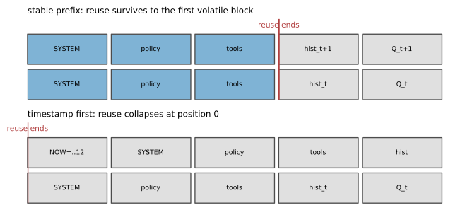
The economics follow. With stable-prefix tokens S, volatile-suffix tokens V, uncached input cost u per token, and a discounted cached-read cost r per token, a later hit costs C_{\text{hit}}=rS+uV while breaking the prefix costs C_{\text{miss}}=u(S+V).
economics = cache_cost(stable_tokens=7000, volatile_tokens=300, read_rate=0.10)
print(f"hit cost:   {economics['hit']:.0f} units")
print(f"miss cost:  {economics['miss']:.0f} units")
print(f"a broken prefix costs {economics['multiplier']:.1f}x as much input work")
hit cost: 1000 units
miss cost: 7300 units
a broken prefix costs 7.3x as much input workAt these illustrative units — S=7000, V=300, cached-read discount r=0.1 — a broken prefix costs 7.3 times the input work of a hit. These are not provider prices; the example isolates a multiplier. This is also the durable core of the Manus lesson on building agents: because the KV cache keys on an exact prefix, prefix stability is the highest-leverage cost control an agent harness has, which is why appending to the context beats editing it and why a single volatile token near the front can silently multiply the bill (Ji 2025). Log the server’s own cached-read and cache-write counts; a local common-prefix count is a diagnostic, not proof of a server hit, because model revision, tokenizer, template, routing, and cache lifetime all intervene.
Prompt caches and server-side context editing share a principle, not one API. As of 2026-07-20, providers expose exact-prefix caching with different thresholds, price discounts, lifetimes, and usage fields; some now offer server-side or SDK-assisted context management (clearing old tool results, compaction hooks) whose defaults, beta headers, and preservation rules differ and change. A cache API does not remove the caller’s obligation to keep a stable prefix, and a context-editing API does not remove the obligation to define what must survive. Keep a model-capability profile beside prompt configuration and gate every migration with the target evaluation suite. Verify live: the current prompt-caching and context-management guides for the exact model you serve, confirmed against usage telemetry (checked 2026-07-20).
13.8 Compaction, just-in-time loading, and the context ledger
A long-running interaction eventually approaches its budget. Dropping the oldest message is simple and unsafe; summarizing everything into one paragraph is compact and unauditable. Good compaction classifies state by survival requirement before it transforms anything: extract the specifications, decisions, open questions, and unresolved errors that must survive verbatim, summarize only the expendable middle, keep the most recent turns, and then assert that the durable items still appear literally. Figure 13.7 makes that survival check an explicit gate that can reject a compaction.
flowchart TD
    U["utilization crosses the trigger at a turn boundary"] --> K["classify decisions, open questions, errors, references"]
    K --> P["pin durable state verbatim"]
    K --> M["summarize the expendable middle"]
    K --> R["keep recent turns"]
    P --> V{"survival assertions pass?"}
    M --> V
    R --> V
    V -- "no" --> F["reject and surface a typed failure"]
    V -- "yes" --> N["emit a labelled compacted state"]
# @save
DURABLE_PREFIXES = ("DECISION ", "OPEN ", "ERROR ")


def assert_survival(before: Sequence[str], after: Sequence[str]) -> None:
    """Fail closed unless every pre-compaction decision and open question survives.

    Literal substring survival is stronger than a model grader for these fields
    and far cheaper to debug: a decision or open question that vanished from the
    compacted transcript is a hard error, not a quality regression.

    Args:
        before: The full transcript before compaction.
        after: The compacted transcript.

    Raises:
        AssertionError: If any ``DECISION`` or ``OPEN`` line is missing from
            ``after``.
    """
    joined = "\n".join(after)
    missing = [m for m in before if m.startswith(("DECISION ", "OPEN ")) and m not in joined]
    if missing:
        raise AssertionError(f"compaction lost durable state: {missing}")


def compact_history(messages: Sequence[str], budget: int, trigger: float = 0.65,
                    keep_recent: int = 4) -> tuple[list[str], bool]:
    """Compact a transcript by classifying durable state before summarizing the rest.

    The rule to take away: never summarize first. Extract the state that must
    survive verbatim (decisions, open questions, errors), summarize only the
    expendable middle, keep the recent turns, then assert survival. Compaction
    fires only when utilization crosses ``trigger``, leaving headroom for the
    next turn, tool results, and output.

    Args:
        messages: The full ordered transcript, oldest first.
        budget: The whitespace-token proxy budget for the active window.
        trigger: Fraction of ``budget`` at which compaction fires.
        keep_recent: Number of most-recent messages kept verbatim.

    Returns:
        A tuple ``(compacted, changed)``; ``changed`` is False when the
        transcript already fit and nothing was rewritten.

    Raises:
        AssertionError: If a durable decision or open question would be lost.
    """
    if token_count("\n".join(messages)) <= budget * trigger:
        return list(messages), False
    durable = [m for m in messages if m.startswith(DURABLE_PREFIXES)]
    recent = list(messages[-keep_recent:])
    omitted = len(messages) - len({*durable, *recent})
    summary = f"SUMMARY: {omitted} routine messages folded; no durable state added."
    compacted = [*durable, summary, *[m for m in recent if m not in durable]]
    assert_survival(messages, compacted)
    return compacted, True


def synthetic_history(turns: int = 40) -> list[str]:
    """Build a debugging trace with sparse, high-value durable state to compact.

    Most turns are routine chatter; a handful carry ``DECISION``, ``OPEN``, and
    ``ERROR`` lines, so the compactor has real durable state to preserve.

    Args:
        turns: Total number of messages in the trace.

    Returns:
        The ordered transcript, oldest message first.
    """
    anchors = {
        5: "DECISION D1: preserve typed tool results; correlation IDs are evidence.",
        11: "OPEN Q1: reproduce the timeout under the production proxy.",
        18: "DECISION D2: retry at most twice; duplicate writes are unsafe.",
        24: "ERROR E1: proxy closed the stream before the tool result arrived.",
        30: "OPEN Q2: confirm whether order writes are idempotent.",
        34: "DECISION D3: pin schema version v4; replay depends on it.",
    }
    return [anchors.get(t, f"TURN {t:02d}: inspected a routine trace batch " + "detail " * 10).strip()
            for t in range(1, turns + 1)]
Compact a 40-message trace whose durable state is six lines buried in routine chatter, and measure utilization before and after against a 500-token proxy budget.
history = synthetic_history()
before_tokens = token_count("\n".join(history))
compacted, changed = compact_history(history, budget=500)
after_tokens = token_count("\n".join(compacted))

print(f"messages: {len(history)} -> {len(compacted)}   changed={changed}")
print(f"tokens:   {before_tokens} -> {after_tokens}")
print(f"utilization: {before_tokens / 500:.3f} -> {after_tokens / 500:.3f}")
print("survivors:")
for message in compacted:
    print("  ", message[:64])
messages: 40 -> 11 changed=True
tokens: 636 -> 135
utilization: 1.272 -> 0.270
survivors:
DECISION D1: preserve typed tool results; correlation IDs are ev
OPEN Q1: reproduce the timeout under the production proxy.
DECISION D2: retry at most twice; duplicate writes are unsafe.
ERROR E1: proxy closed the stream before the tool result arrived
OPEN Q2: confirm whether order writes are idempotent.
DECISION D3: pin schema version v4; replay depends on it.
SUMMARY: 30 routine messages folded; no durable state added.
TURN 37: inspected a routine trace batch detail detail detail de
TURN 38: inspected a routine trace batch detail detail detail de
TURN 39: inspected a routine trace batch detail detail detail de
TURN 40: inspected a routine trace batch detail detail detail deThe transcript falls from over budget to a quarter of it, and every DECISION, OPEN, and ERROR line survives verbatim beside a single summary of the folded middle. A summary that quietly turned “do not deploy” into “deploy later,” or “timeout occurred” into “timeout fixed,” would poison every later turn; the literal survival check is what makes that a caught error rather than a silent one. Record the compactor version, input and output digests, trigger reason, and preserved-item counts, and treat the compacted block as an application-produced summary — not developer policy, not verbatim user speech.
The other budget lever is loading less to begin with. Preloading every manual and tool description pays input cost on every call; just-in-time loading keeps compact references and resolves a subset when the task provides enough scent. If N documents average L tokens, preloading costs about NL; loading k\ll N plus an index of I tokens costs
C_{\text{JIT}}=I+kL. \tag{13.5}
The saving NL-(I+kL) is real but selection is not free — it adds latency, can miss the needed item, and may need another round trip. Preload the small stable contract needed on nearly every call; use JIT for a large catalog with sparse per-call use; and give references enough scent (a name, a purpose, a constraint) that the selector can choose, because a list of opaque ids has none. This is also the Manus discipline for tools: keep the definitions stable and mask the ones a step may not use rather than removing them, so the prefix — and its cache — stays intact, and recite the evolving plan into recent context so the goal does not decay across a long trajectory (Ji 2025).
None of this is operable without a context ledger — one record per call that makes every segment’s presence reconstructable.
| Field | Question it answers |
|---|---|
| model, template, prompt, assembler versions | which executable configuration ran? |
| segment kind, source, trust, digest, token count | what entered, from where, under whose authority? |
| selection reason and score | why was this item chosen? |
| position and truncation outcome | where did it land, and what was omitted? |
| input budget and utilization | how close was the call to its envelope? |
| cached-read and cache-write tokens | did the expected prefix actually reuse? |
| compaction event and preserved-state counts | what changed between turns? |
| output usage, latency, cost, evaluation outcome | what did the context buy? |
We close by exercising compaction and prefix stability together, because they solve different constraints and must not be conflated. The simulation grows a transcript over 50 turns, crossing compaction on/off with a stable/broken prefix, and records utilization and reusable-prefix fraction per turn — using the same survival-checked compactor, on a history that contains real durable lines.
# @save
POLICY_TOKENS = 600
STABLE_POLICY = "SYSTEM\n" + "stable-policy-token " * POLICY_TOKENS


def simulate_turns(compaction: bool, stable_prefix: bool, turns: int = 50,
                   budget: int = 1100) -> list[dict]:
    """Grow a transcript turn by turn, recording utilization and reusable-prefix fraction.

    Each turn appends an observation (with occasional durable decision, open
    question, and error lines); with ``compaction`` on, the survival-checked
    ``compact_history`` runs at a clean boundary. With ``stable_prefix`` off, a
    changing timestamp is prepended, which breaks cache reuse at byte 0. The two
    controls are independent: compaction bounds utilization, a stable prefix
    preserves reuse, and neither substitutes for the other.

    Args:
        compaction: Whether to compact when history crosses the trigger.
        stable_prefix: Whether the leading bytes stay identical across turns.
        turns: Number of turns to simulate.
        budget: The whitespace-token proxy budget for the whole window.

    Returns:
        One ledger row per turn with tokens, utilization, reuse fraction, and a
        compaction flag.
    """
    anchors = {8: "DECISION D1: route delivery failures to status, not refund.",
               15: "OPEN Q1: does the refund tool need a second approval?",
               22: "ERROR E1: tool timeout on the refund path.",
               31: "DECISION D2: cap auto-refunds at two per account per day.",
               40: "OPEN Q2: is the shipment webhook idempotent?"}
    history, previous, ledger = [], "", []
    history_budget = budget - token_count(STABLE_POLICY)
    for turn in range(1, turns + 1):
        history.append(anchors.get(turn, f"TURN {turn:02d} observation " + "working-token " * 20))
        did_compact = False
        if compaction:
            history, did_compact = compact_history(history, history_budget,
                                                    trigger=0.65, keep_recent=3)
        body = STABLE_POLICY + "\n" + "\n".join(history)
        prompt = body if stable_prefix else f"NOW=2026-07-20T12:00:{turn:02d}Z\n{body}"
        reusable = common_prefix_bytes(previous, prompt) if previous else 0
        ledger.append({"turn": turn, "tokens": token_count(prompt),
                       "utilization": token_count(prompt) / budget,
                       "reuse": reusable / len(prompt.encode("utf-8")),
                       "compacted": did_compact})
        previous = prompt
    return ledger
grid = {(comp, stab): simulate_turns(comp, stab)
for comp in (False, True) for stab in (True, False)}
for (comp, stab), rows in grid.items():
tag = f"compaction={'on' if comp else 'off':3}, prefix={'stable' if stab else 'broken'}"
max_util = max(r["utilization"] for r in rows)
mean_reuse = sum(r["reuse"] for r in rows[1:]) / (len(rows) - 1)
events = sum(r["compacted"] for r in rows)
print(f"{tag:34} max_util={max_util:.3f} mean_reuse={mean_reuse:.3f} events={events}")compaction=off, prefix=stable max_util=1.527 mean_reuse=0.985 events=0
compaction=off, prefix=broken max_util=1.528 mean_reuse=0.001 events=0
compaction=on , prefix=stable max_util=0.839 mean_reuse=0.977 events=4
compaction=on , prefix=broken max_util=0.840 mean_reuse=0.002 events=4The grid separates the two axes cleanly, and Figure 13.8 plots them.
Show the code that draws this figure
styles = {(False, True): ("off / stable", "-", "o"), (True, True): ("on / stable", "-", "s"),
          (False, False): ("off / broken", "--", "o"), (True, False): ("on / broken", "--", "s")}
fig, (ax1, ax2) = plt.subplots(1, 2, figsize=(7.8, 3.2))
for key, rows in grid.items():
    label, ls, mk = styles[key]
    turns = [r["turn"] for r in rows]
    ax1.plot(turns, [r["utilization"] for r in rows], ls=ls, label=label)
    ax2.plot(turns[1:], [r["reuse"] for r in rows[1:]], ls=ls, label=label)
ax1.axhline(1.0, color="0.5", ls=":")
ax1.set_xlabel("turn"); ax1.set_ylabel("context utilization"); ax1.legend(fontsize=7)
ax2.set_xlabel("turn"); ax2.set_ylabel("reusable-prefix fraction"); ax2.legend(fontsize=7)
fig.tight_layout()
plt.show()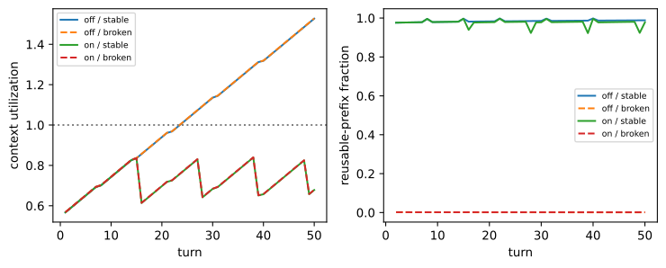
Without compaction, utilization runs well past 1.0; with it, utilization stays bounded below its trigger envelope while every durable line still survives. Orthogonally, the stable-prefix runs keep almost all leading bytes reusable and the timestamp-first runs keep almost none — and a compaction event, which rewrites the middle, does not destroy the stable base. Context pressure and prefix reuse are independent constraints solved by independent controls, and the ledger is what lets an operator see both at once. Chapter 14 takes selected external evidence as its own subject, building retrieval and ranking rather than asking this assembler to improvise them; the handoff is clean, because R in Equation 13.3 arrives already scored and provenance-tagged.
13.9 Summary
A prompt is executable, model-scoped configuration, and improving it requires a frozen distribution and a metric — the failure table, not the scalar, is where measurement starts. Demonstrations are a dataset in the prompt that can help or hurt, and automatic optimization generates candidates from failure traces but overfits a small dev split exactly as training overfits weights. Context is a constructed input: typed, ordered, trust-labelled segments under a budget, never a growing transcript. Structure aids parsing but does not create trust; a stable prefix is a caller-side cache invariant; compaction must classify durable state before summarizing and assert survival. Chapter 14 supplies the retrieved evidence this assembler places.
13.10 Exercises
Read the failure table, then fix one class. Run
evaluate(BASELINE, DEV_SET)and group the failures by their(expected, actual)confusion. Change only theprecedenceof aPromptand re-score. Which failures does precedence fix, which does it leave, and why is the cue-less refund case immune to any precedence order?Corrupt a demonstration. Using
classify, build a two-demonstration prompt where one demonstration is correctly labelled and one is corrupted. (a) Find a query that the corruption flips and one it does not, and explain the flip in terms of_similarity. (b) Lowerdemo_thresholdand describe what breaks. (c) Argue when a static demonstration set is safer than query-dependent selection.Push the optimizer to overfit further. Extend
HELDOUT_SETwith two refund tickets phrased unlike any dev case, then re-runoptimize_prompt. Report the final dev and held-out scores and the round at which they diverge. What promotion rule, defined before the search, would have rejected the winner?Make truncation fail loudly. Construct a segment list where a required tool schema and the query together exceed the budget. Show that
render_contextraises rather than dropping either, then redesign the segments (usingselect_contextand awrite-style reference) so the call fits without losing the query.Attack compaction semantically. Build a 30-message trace containing a negation (“do not deploy”), a superseded decision, two similar order ids, and a tool result whose units matter. Design a survival check stronger than substring matching for at least one of these, then exhibit a summary that passes a generic quality judge but fails your check.
Compute and defend a JIT boundary. A catalog has 400 tools averaging 180 description tokens; a compact index costs 4,000 tokens and an average call uses five tools. Use Equation 13.5 to compute preload and JIT input sizes, then write a short memo that names the lookup latency, selection recall, cache reuse, and cost-of-omission that would move your decision either way.
Add a third prefix policy. Extend
simulate_turnswith a variant that changes one tool description every tenth turn. Plot utilization, reusable-prefix fraction, and compaction events for all three policies, and write an alert rule that fires on an unexpected prefix regression without firing on a planned tool-description release.