# @save
from dataclasses import dataclass

import torch
from torch import Tensor, nn
from torch.nn import functional as F


@dataclass
class RoutingState:
    """Everything a caller needs to mix experts and to diagnose balance.

    A single forward pass returns the full score distribution, the selected
    experts with their normalized gates, the measured per-expert load, and the
    two balancing losses, so nothing about a routing decision is hidden.

    Args:
        probabilities: Scores over all experts, shape ``(..., E)``.
        weights: Normalized gates for the selected experts, ``(..., k)``.
        indices: Selected expert ids, ``(..., k)``.
        load: Fraction of routed slots each expert received, ``(E,)``.
        balance_loss: Switch-style auxiliary load-balance loss (scalar).
        z_loss: Router z-loss penalizing oversized logits (scalar).
    """

    probabilities: Tensor
    weights: Tensor
    indices: Tensor
    load: Tensor
    balance_loss: Tensor
z_loss: Tensor4 Mixture-of-Experts and Efficient Architectures
A frontier agent model is often described with two numbers: “one trillion parameters, 32 billion active.” Both are true, and they answer different engineering questions. The trillion parameters set how much learned capacity exists and how much weight storage the serving fleet must hold. The 32 billion active approximate how many weights actually touch a single token on its way through the network. A dense feed-forward network — the token-wise MLP we put in every TinyGPT block back in ?sec-ch02-block — applies all of its parameters to every token, so for it the two numbers are equal. This chapter is about the architectures that pull them apart, and about a second split just like it on the sequence axis, where Section 3.1 showed KV state growing with every token.
We build the mechanisms in small executed pieces and read their economics off real files: (i) a top-k router that turns one dense FFN into conditional compute, run on a batch with its shapes printed; (ii) the two parameter ledgers — stored and active — computed for a worked layer; (iii) a routing-collapse demo that trains a toy MoE with and without a load-balancing term and watches expert utilization live; (iv) a gated linear-attention block whose recurrent state stays fixed no matter how long the sequence, plus the S4-to-Mamba lineage it belongs to; (v) a recall probe that measures exactly what that fixed state costs; and (vi) a config parser that reconstructs total and active parameters, and 32K-token state, for three published models — a dense one, an MoE, and a linear/full hybrid. Two questions organize the work: which parameters process a token, and how sequence history is stored.
4.1 Routing turns a dense FFN into conditional compute
A dense FFN sends every token through the same large matrices. A mixture-of-experts (MoE) layer instead stores many FFNs — the experts — and sends each token to only a few of them. The idea predates Transformers, but the sparsely-gated MoE layer made it practical at language scale (Shazeer et al. 2017), and GShard and Switch Transformers carried it to production models (Lepikhin et al. 2020; Fedus et al. 2022). Adding experts grows total capacity while the number each token uses stays fixed. The price is a new learned component — the router — that must decide, per token, which experts to consult.
Let x\in\mathbb{R}^d be one token’s representation and E_i(x) expert i’s FFN. The router is a single linear map producing one logit per expert, r=W_r x. We turn logits into scores p (softmax, so experts compete; or independent sigmoids), keep the indices I(x) of the k largest, and mix only those experts, reweighted by their gates:
y=\sum_{i\in I(x)} g_i\,E_i(x), \qquad g_i=\frac{p_i}{\sum_{j\in I(x)}p_j}. \tag{4.1}
The normalization runs over the selected experts, so the gates of the winners sum to one. Selection is discrete: gradients reach W_r through the kept gate values and through the balancing terms we add next, never through the top-k index operation itself. We write the router as a module that also exposes the diagnostics we will need to debug it.
The forward pass is Equation 4.1 plus the observables. load is the fraction of routed slots each expert won (it sums to one); balance_loss and z_loss are defined in the next section — we compute them here so every routing decision carries its own diagnostics.
# @save
class TopKRouter(nn.Module):
    """Score each token over ``experts`` experts and keep the top ``top_k``.

    The router is one linear map from width ``d`` to ``E`` logits. A separate
    ``selection_bias`` buffer steers *which* experts win (the aux-loss-free
    controller writes it) without touching the output gates, keeping the "who
    computes" and "how much they count" decisions cleanly apart.

    Args:
        width: Token width ``d``.
        experts: Number of experts ``E``.
        top_k: Experts selected per token ``k``.
        scoring: ``"softmax"`` for competing scores, ``"sigmoid"`` for
            independent ones.
    """

    def __init__(self, width: int, experts: int, top_k: int, scoring: str = "softmax") -> None:
        super().__init__()
        if not 1 <= top_k <= experts or scoring not in {"softmax", "sigmoid"}:
            raise ValueError("invalid top_k or scoring function")
        self.experts, self.top_k, self.scoring = experts, top_k, scoring
        self.projection = nn.Linear(width, experts)
        self.register_buffer("selection_bias", torch.zeros(experts))

    def forward(self, tokens: Tensor) -> RoutingState:
        logits = self.projection(tokens)
        probabilities = logits.softmax(-1) if self.scoring == "softmax" else logits.sigmoid()
        indices = (probabilities + self.selection_bias).topk(self.top_k, dim=-1).indices
        weights = probabilities.gather(-1, indices)
        if self.top_k > 1:
            weights = weights / weights.sum(-1, keepdim=True).clamp_min(1e-9)
        flat = indices.reshape(-1, self.top_k)
        load = F.one_hot(flat, self.experts).float().sum(1).mean(0) / self.top_k
        mean_probability = probabilities.reshape(-1, self.experts).mean(0)
        balance_loss = self.experts * (load.detach() * mean_probability).sum()
        z_loss = logits.logsumexp(-1).square().mean()
        return RoutingState(probabilities, weights, indices, load, balance_loss, z_loss)

    @torch.no_grad()
    def update_selection_bias(self, load: Tensor, rate: float = 1e-2) -> None:
        """Nudge each expert's bias toward uniform load (aux-loss-free control).

        Overloaded experts get their bias lowered and underloaded ones raised by
        a fixed step; subtracting the mean keeps the biases from drifting as a
        group, since only their differences change the selection.

        Args:
            load: Measured per-expert routed fraction, ``(E,)``.
            rate: Step size for the sign update.
        """
        target = torch.full_like(load, 1 / self.experts)
        self.selection_bias.add_(rate * torch.sign(target - load))
        self.selection_bias.sub_(self.selection_bias.mean())
Run it on a tiny batch. With four experts, top-2 routing, and six tokens, the router should return a score per expert, two indices and two gates per token, and a load vector that sums to one.
torch.manual_seed(0)
router = TopKRouter(width=8, experts=4, top_k=2)
tokens = torch.randn(2, 3, 8)  # batch 2, length 3, width 8
state = router(tokens)
print("probabilities:", tuple(state.probabilities.shape))
print("indices:      ", tuple(state.indices.shape), "  weights:", tuple(state.weights.shape))
print("token[0,0] -> experts", state.indices[0, 0].tolist(),
      "gates", [round(w, 3) for w in state.weights[0, 0].tolist()],
      "(sum", round(state.weights[0, 0].sum().item(), 3), ")")
print("per-expert load:", [round(x, 3) for x in state.load.tolist()],
      "sum", round(state.load.sum().item(), 3))
probabilities: (2, 3, 4)
indices: (2, 3, 2) weights: (2, 3, 2)
token[0,0] -> experts [1, 3] gates [0.52, 0.48] (sum 1.0 )
per-expert load: [0.25, 0.333, 0.167, 0.25] sum 1.0The shapes confirm the contract: a (2, 3, 4) score tensor, (2, 3, 2) indices and gates, the two gates summing to one, and a four-element load that sums to one. Figure 4.1 traces that path for a single token — the mechanism at the heart of every MoE layer.
flowchart LR
    X["token x"] --> R["router W_r x"]
    R --> S["scores over E=4 experts"]
    S --> T["top-k select (k=2)"]
    T --> E1["expert 1"]
    T --> E3["expert 3"]
    E1 --> C["combine: g1*E1 + g3*E3"]
    E3 --> C
    C --> Y["output y"]
    S -.->|not selected| E0["experts 0,2 idle"]
Routing is per token, not per sequence: two adjacent tokens can pick different experts, and one expert may see tokens from unrelated topics. Visualizations sometimes reveal statistical specialization, but expert ids are not guaranteed to be human-readable job titles. The dependable contract is behavioral — the router picks the parameter subset that best reduces the loss under whatever balance pressure we apply.
4.2 The two parameter ledgers
Now we can make “total versus active” precise. A SwiGLU-style expert of width d and intermediate width h_e holds three dominant matrices — gate-up, value-up, and down — for roughly
P_e \approx 3\,d\,h_e \tag{4.2}
parameters. A layer that stores E routed experts, selects k, and always runs S shared experts has two ledgers: everything stored, and the subset a token touches.
P_{\text{stored}}=(E+S)\,P_e, \qquad P_{\text{active}}=(k+S)\,P_e. \tag{4.3}
Take a concrete layer — width {4096}, {64} experts of intermediate width {1024}, top-2, one shared expert — and compute both ledgers instead of trusting a ratio.
d, E, k, S, h_e = 4096, 64, 2, 1, 1024  # width, routed experts, selected, shared, expert width
P_e = 3 * d * h_e
stored = (E + S) * P_e
active = (k + S) * P_e
print(f"per-expert P_e = 3*d*h_e = {P_e:,}")
print(f"stored  (E+S)*P_e = {stored:,}")
print(f"active  (k+S)*P_e = {active:,}")
print(f"active fraction of the expert bank = {active / stored:.2%}")
print(f"the naive k/E guess would say       = {k / E:.2%}")
per-expert P_e = 3*d*h_e = 12,582,912
stored (E+S)*P_e = 817,889,280
active (k+S)*P_e = 37,748,736
active fraction of the expert bank = 4.62%
the naive k/E guess would say = 3.12%The active fraction is 4.6%, not the 3.1% that k/E suggests. The shared expert runs for every token, so it is counted in both ledgers — it lifts the active fraction above the naive ratio. And this is only the expert bank. Attention, embeddings, the output head, layer norms, the router itself, and any dense-first layers are active for every token too; in a fine-grained MoE that common trunk can be a large slice of the active count. Figure 4.2 shows the split for this layer.
Show the code that draws this figure
import matplotlib.pyplot as plt

fig, ax = plt.subplots(figsize=(5.6, 3.6))
ax.bar(["stored\n(E+S)", "active\n(k+S)"], [stored / 1e6, active / 1e6],
       color=["#c9ced6", "#2a7f9e"])
ax.set_ylabel("expert parameters (millions)")
for i, val in enumerate([stored, active]):
    ax.text(i, val / 1e6, f"{val/1e6:.0f}M", ha="center", va="bottom")
fig.tight_layout()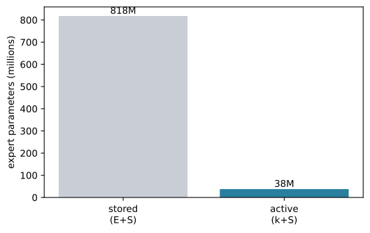
Two more distinctions keep the ledgers honest. Parameter count is not FLOPs — activations, attention, and normalization all add compute the ledger ignores. And active count is not resident memory: if every expert must be reachable at low latency, its weights exist somewhere in the serving topology whether or not a given token uses them. Quantization shrinks their bytes and offloading trades memory for transfers, but neither changes the logical total.
4.3 Balance is the optimization problem
A router that starts with a slight preference can dig itself into a hole. The favored expert sees more tokens, so it gets more gradient, so it becomes more useful, so it wins even more tokens. The others starve. This routing collapse wastes most of the stored parameters and, on a real cluster, overloads one device while the rest idle. The fix is to add pressure toward uniform use. Two statistics separate probability mass from actual assignments. For expert i over N tokens,
f_i=\frac{1}{Nk}\sum_{n}\mathbf{1}[i\in I(x_n)], \qquad P_i=\frac{1}{N}\sum_{n}p_i(x_n), \tag{4.4}
the hard routed fraction and the mean soft score. The Switch-style auxiliary loss multiplies them, L_{\text{balance}}=E\sum_i f_i P_i (Fedus et al. 2022); because f_i is discrete it is detached, and the differentiable P_i supplies the gradient that spreads tokens out. To see collapse and its cure, we wrap the router in a small MoE classifier and deliberately bias expert 0 at initialization.
# @save
class ToyMoE(nn.Module):
    """A local top-1 MoE classifier used to demonstrate routing collapse.

    Experts are tiny MLPs and dispatch is a plain Python loop over experts —
    no expert-parallel communication — so the training dynamics of the router,
    not systems throughput, are what this model exposes.

    Args:
        width: Input width.
        experts: Number of routed experts.
        hidden: Per-expert hidden width.
        classes: Output classes.
    """

    def __init__(self, width: int = 8, experts: int = 4, hidden: int = 16, classes: int = 4) -> None:
        super().__init__()
        self.router = TopKRouter(width, experts, top_k=1)
        self.classes = classes
        self.experts = nn.ModuleList(
            nn.Sequential(nn.Linear(width, hidden), nn.SiLU(), nn.Linear(hidden, classes))
            for _ in range(experts)
        )

    def forward(self, tokens: Tensor) -> tuple[Tensor, RoutingState]:
        routing = self.router(tokens)
        flat = tokens.reshape(-1, tokens.size(-1))
        indices = routing.indices.reshape(-1, 1)
        weights = routing.weights.reshape(-1, 1)
        out = flat.new_zeros(flat.size(0), self.classes)
        for slot in range(routing.indices.size(-1)):
            for expert_id, expert in enumerate(self.experts):
                rows = torch.where(indices[:, slot] == expert_id)[0]
                if rows.numel():
                    out[rows] += weights[rows, slot, None] * expert(flat[rows])
        return out.view(*tokens.shape[:-1], self.classes), routing
The training loop is ordinary supervised learning with one extra term: balance_weight * balance_loss. Setting that weight to zero lets collapse run its course; setting it to 0.5 fights back.
# @save
def train_router(balance_weight: float, steps: int = 300) -> dict[str, object]:
    """Train the toy MoE with a chosen load-balance weight and report the result.

    Expert 0 is biased at initialization so that, with no balancing pressure,
    the router collapses onto it; the balance term is the only thing that can
    reopen the other experts, which is exactly the effect we want to isolate.

    Args:
        balance_weight: Coefficient on the auxiliary load-balance loss.
        steps: Optimizer steps.

    Returns:
        A dict with the held-out per-expert ``load``, task ``accuracy``, and the
        two router losses.
    """
    torch.manual_seed(5)
    torch.set_num_threads(1)
    model = ToyMoE()
    nn.init.zeros_(model.router.projection.weight)
    nn.init.constant_(model.router.projection.bias, -1.0)
    model.router.projection.bias.data[0] = 2.0  # expert 0 starts favored
    optimizer = torch.optim.Adam(model.parameters(), lr=2e-2)
    generator = torch.Generator().manual_seed(8)
    for _ in range(steps):
        batch = torch.randn(256, 8, generator=generator)
        labels = batch[:, :4].argmax(-1)
        logits, routing = model(batch)
        loss = (F.cross_entropy(logits, labels)
                + balance_weight * routing.balance_loss
                + 1e-4 * routing.z_loss)
        optimizer.zero_grad()
        loss.backward()
        optimizer.step()
    with torch.no_grad():
        batch = torch.randn(8_192, 8, generator=generator)
        labels = batch[:, :4].argmax(-1)
        logits, routing = model(batch)
    return {"balance_weight": balance_weight, "load": routing.load.tolist(),
            "accuracy": (logits.argmax(-1) == labels).float().mean().item(),
            "balance_loss": routing.balance_loss.item(), "z_loss": routing.z_loss.item()}
We run both conditions and print the held-out load and accuracy.
unbalanced = train_router(balance_weight=0.0)
balanced = train_router(balance_weight=0.5)
print("unbalanced load:", [round(x, 4) for x in unbalanced["load"]],
      " accuracy", round(unbalanced["accuracy"], 4))
print("balanced   load:", [round(x, 4) for x in balanced["load"]],
      " accuracy", round(balanced["accuracy"], 4))
unbalanced load: [1.0, 0.0, 0.0, 0.0] accuracy 0.9835
balanced load: [0.2657, 0.2305, 0.2456, 0.2582] accuracy 0.9734Without the balance term the router sends 100% of held-out tokens to expert 0 and the other three are dead — yet task accuracy is 98.3%, because a single expert is enough for this easy toy task. That is the trap: the loss looks healthy while most of the model is wasted. With balance_weight=0.5 the loads land near 26/23/25/26% and accuracy is 97.3% — a hair lower, because balancing pressure competes with the task. Figure 4.3 draws both.
Show the code that draws this figure
fig, axes = plt.subplots(1, 2, figsize=(7.2, 3.3), sharey=True)
for ax, run, title in [(axes[0], unbalanced, "no balancing"), (axes[1], balanced, "balance weight 0.5")]:
    ax.bar(range(4), run["load"], color="#a14f3b" if run is unbalanced else "#2a7f9e")
    ax.axhline(0.25, color="#555", ls="--", lw=1)
    ax.set(title=title, xlabel="expert", xticks=range(4), ylim=(0, 1.05))
axes[0].set_ylabel("fraction of routed tokens")
fig.tight_layout()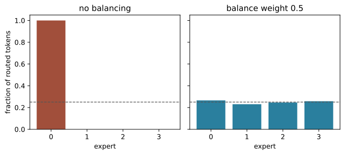
A production run stacks two more controls on top of the auxiliary loss. Router logits can drift to unstable magnitudes, so ST-MoE added a z-loss, L_z=\frac1N\sum_n(\log\sum_i e^{r_i(x_n)})^2, that keeps the log-partition small; it is a numerical-stability tool, not a balancer (Zoph et al. 2022). And balancing need not live in the task loss at all. DeepSeek-V3 keeps a per-expert selection bias b_i, routes on p_i+b_i, and after each step lowers the bias of overloaded experts and raises it for underloaded ones — the update_selection_bias method above (DeepSeek-AI 2024). One control step makes the direction visible.
controller = TopKRouter(4, experts=4, top_k=1)
controller.update_selection_bias(torch.tensor([0.70, 0.10, 0.10, 0.10]), rate=0.02)
print("bias after one step:", [round(x, 4) for x in controller.selection_bias.tolist()])
bias after one step: [-0.03, 0.01, 0.01, 0.01]The overloaded expert 0 gets a negative bias and the three starved experts a positive one, with the mean held at zero — pure feedback control, no gradient through the task. Whichever mechanism a model uses, the operational lesson is the same: a low training loss does not prove healthy expert use, so balance must be measured, per layer, as load, entropy, and the busiest-versus-median gap.
4.4 The MoE design space and its systems tax
“An MoE” leaves several knobs unset, and each has a concrete consequence. Granularity: a coarse MoE stores a few wide experts; a fine-grained one splits the same capacity into many small experts and selects several — choosing 8 of 256 is a far richer code than 1 of 8, but each expert then sees fewer tokens per step, so its matmuls shrink and its training gets noisier. Selected count k: top-1 is cheapest; top-2 or more mixes experts like a small ensemble at higher active cost. Shared path: a shared expert gives every token a dense route for common transformations, at the cost of appearing in every active-parameter count (Section 4.2). Placement: if only every fourth FFN is sparse, three-quarters of the FFN layers are dense; if the first layers are dense-first, their parameters are always active. A model name like A3B encodes one publisher’s counting convention, not a number you can rederive without knowing which of these are included.
The tax that has no analog in a dense model begins right after top-k. Under expert parallelism each device owns a subset of experts, but a token’s chosen experts may live on other devices. A conceptual MoE layer therefore becomes a communication pipeline, drawn in Figure 4.4: score and assign, permute tokens by destination, exchange them (an all-to-all collective), run the local expert matmuls, exchange the outputs back, and recombine by gate. Small experts turn compute into communication; skew makes some devices stragglers; padding wastes bandwidth while variable sizes complicate scheduling; and crossing a node boundary costs more than moving within one accelerator. This is why two models with equal active-parameter counts can have very different latency. The kernels and placement that tame it belong to Chapters 6 and 10; the durable rule here is that conditional FLOPs are not free when the chosen weights or tokens are far away.
Capacity planning inherits the same split. Communication kernels often cap each expert at C=\lceil c\,Nk/E\rceil tokens for a capacity factor c\ge 1; beyond C the system drops tokens, reroutes them, or uses a dropless variable-size dispatch. A quick calculation shows why skew hurts even with generous capacity.
N, experts, k, c = 8_192, 32, 2, 1.25
capacity = -(-int(c * N * k) // experts)  # ceil(c * N * k / E)
hot_share = 0.30  # one expert grabs 30% of assignments
hot_tokens = int(hot_share * N * k)
dropped = max(0, hot_tokens - capacity)
print(f"per-expert capacity C = {capacity}")
print(f"a hot expert wants {hot_tokens} tokens -> {dropped} dropped under static capacity")
per-expert capacity C = 640
a hot expert wants 4915 tokens -> 4275 dropped under static capacityEven at a 1.25 capacity factor, a single expert that attracts 30% of assignments overflows its buffer by thousands of tokens, all of which are dropped — computed for nothing, and worse for quality if they were important. Balance is thus simultaneously an optimization target and a systems constraint.
4.5 Linear attention and state-space models change memory
MoE sparsifies which parameters touch a token. The second efficiency axis changes how sequence history is stored. Recall from Section 3.1 that softmax attention keeps a key and value for every past token, so the KV cache grows linearly with context. Linear attention removes the softmax so the sums can be reassociated: replace the similarity \text{sim}(q,k) with a factored feature map \phi(q)^\top\phi(k), and the causal computation collapses into a running state that is updated, not appended:
S_t=\lambda_t\,S_{t-1}+\phi(k_t)\,v_t^{\top}, \qquad z_t=\lambda_t\,z_{t-1}+\phi(k_t), \qquad y_t=\frac{\phi(q_t)^\top S_t}{\phi(q_t)^\top z_t+\epsilon}. \tag{4.5}
Here S_t has shape m\times d_v (feature width by value width) and z_t has width m — both independent of t. The learned decay \lambda_t lets the state forget. We build exactly this recurrence and, crucially, make one block serve two callers: a full parallel sweep over a sequence, and a token-at-a-time streaming mode that carries the state forward. The two must agree.
# @save
class GatedLinearAttention(nn.Module):
    """A linear-attention block whose recurrent state is fixed-size in context.

    Each step folds one token into a running matrix state ``S`` and normalizer
    ``z`` (@eq-ch04-gla), so decoding cost and stored state do not grow with
    sequence length. Passing the returned ``recurrent`` tuple back in resumes
    the scan, so the same weights serve a full-sequence pass and a streaming
    decode.

    Args:
        width: Model width ``d`` (also the value width ``d_v``).
        state_width: Feature width ``m`` of the key/query maps.
    """

    def __init__(self, width: int, state_width: int) -> None:
        super().__init__()
        self.query = nn.Linear(width, state_width, bias=False)
        self.key = nn.Linear(width, state_width, bias=False)
        self.value = nn.Linear(width, width, bias=False)
        self.decay = nn.Linear(width, 1)
        self.output = nn.Linear(width, width, bias=False)

    def forward(self, tokens: Tensor, recurrent: tuple[Tensor, Tensor] | None = None
                ) -> tuple[Tensor, tuple[Tensor, Tensor]]:
        batch, steps, width = tokens.shape
        state_width = self.query.out_features
        if recurrent is None:
            state = tokens.new_zeros(batch, state_width, width)
            normalizer = tokens.new_zeros(batch, state_width)
        else:
            state, normalizer = recurrent
        outputs = []
        for step in range(steps):
            token = tokens[:, step]
            query = F.elu(self.query(token)) + 1  # positive feature map
            key = F.elu(self.key(token)) + 1
            value = self.value(token)
            decay = self.decay(token).sigmoid()
            state = decay[:, :, None] * state + torch.einsum("bf,bd->bfd", key, value)
            normalizer = decay * normalizer + key
            numerator = torch.einsum("bf,bfd->bd", query, state)
            denominator = (query * normalizer).sum(-1, keepdim=True).clamp_min(1e-6)
            outputs.append(self.output(numerator / denominator))
        return torch.stack(outputs, dim=1), (state, normalizer)
We feed a nine-token sequence through the block in one sweep, then again one token at a time, and check the outputs match and the state size is fixed.
torch.manual_seed(7)
gla = GatedLinearAttention(width=12, state_width=5).eval()
sequence = torch.randn(2, 9, 12)
full, _ = gla(sequence)
recurrent, pieces = None, []
for i in range(sequence.size(1)):
    step_out, recurrent = gla(sequence[:, i:i + 1], recurrent)
    pieces.append(step_out)
streamed = torch.cat(pieces, dim=1)
print("full vs streamed max abs diff:", f"{(full - streamed).abs().max().item():.1e}")
print("state scalars 2*(m*d_v + m):", sum(t.numel() for t in recurrent),
      "-> the same at T=9 or T=9,000,000")
full vs streamed max abs diff: 0.0e+00
state scalars 2*(m*d_v + m): 130 -> the same at T=9 or T=9,000,000The streaming path reproduces the full sweep to floating-point roundoff, and the state is 130 scalars whether the sequence is nine tokens or nine million. That constant-state property is the whole point, and Figure 4.5 prices it against the KV cache from Section 3.1.
Show the code that draws this figure
import importlib.util, sys
from pathlib import Path


def _load_chapter(name, relative):
    root = Path.cwd()
    for _ in range(5):
        candidate = root / relative
        if candidate.exists():
            spec = importlib.util.spec_from_file_location(name, candidate)
            module = importlib.util.module_from_spec(spec); sys.modules[name] = module
            spec.loader.exec_module(module); return module
        root = root.parent
    raise FileNotFoundError(relative)


_kv = _load_chapter("ch03_kv_fig", "code/ch03/_generated.py")
cfg = _kv.KVConfig("32L GQA", layers=32, query_heads=32, kv_heads=8, head_dim=128, bytes_per_scalar=2)
lengths = [1_024 * 2 ** i for i in range(8)]
kv_gib = [_kv.kv_bytes(cfg, t) / 2**30 for t in lengths]
recurrent_gib = [32 * (128 * 128) * 2 / 2**30] * len(lengths)  # flat: layers * (m*d_v) * bytes
fig, ax = plt.subplots(figsize=(6.0, 3.6))
ax.plot(lengths, kv_gib, "o-", color="#a14f3b", label="full-attention KV")
ax.plot(lengths, recurrent_gib, "s--", color="#2a7f9e", label="fixed recurrent state")
ax.set(xscale="log", xlabel="context tokens", ylabel="persistent state (GiB)")
ax.legend(frameon=False)
fig.tight_layout()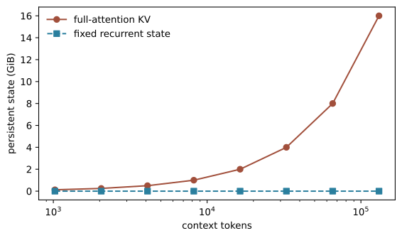
Where does the decay \lambda_t come from, and how expressive can a fixed state be? That is the state-space model (SSM) lineage. A linear SSM writes h_t=A h_{t-1}+B x_t, y_t=C h_t+D x_t; the art is making the recurrence expressive, stable over long horizons, and parallelizable for training. S4 structured A so the equivalent long convolution was cheap (Gu et al. 2022); Mamba made A,B,C input-dependent — the model selects what to keep or forget per token — and supplied a hardware-aware scan (Gu and Dao 2023); Mamba-2 then showed SSMs and attention-like matrix transforms are two views of one object (Dao and Gu 2024). The selective idea is easy to see in one dimension: give the recurrence an input-dependent decay and watch a single impulse either persist or vanish.
def selective_scan(inputs, decays):
    """One-dimensional selective SSM: h_t = a_t * h_{t-1} + x_t."""
    h, history = 0.0, []
    for x, a in zip(inputs, decays):
        h = a * h + x
        history.append(round(h, 3))
    return history


impulse = [1.0, 0.0, 0.0, 0.0, 0.0]
print("slow decay a=0.9 (remembers):", selective_scan(impulse, [0.9] * 5))
print("fast decay a=0.2 (forgets):  ", selective_scan(impulse, [0.2] * 5))
slow decay a=0.9 (remembers): [1.0, 0.9, 0.81, 0.729, 0.656]
fast decay a=0.2 (forgets): [1.0, 0.2, 0.04, 0.008, 0.002]With a=0.9 the impulse is still 0.66 four steps later; with a=0.2 it is gone by the second step. A selective model chooses that decay per token from its content, which is how a fixed-state model keeps a salient fact while discarding filler. The same lineage now includes gated delta networks, which update memory by the difference between a new value and the one currently retrieved (Yang et al. 2024), and recurrent families such as RWKV. The names differ; the fixed-state contract does not.
4.6 Fixed state forces a recall tradeoff
Constant state is a lossy channel. Write n arbitrary key-value pairs, then ask for any one of them. Full attention keeps a separate addressable slot per pair, so it answers exactly. A fixed state must eventually map distinct histories to overlapping representations — without assumptions about the data, exact recall of unbounded independent associations is impossible at fixed precision. The clean way to see this is to isolate the linear-attention memory itself: the same outer-product update S=\sum_i \phi(k_i)v_i^\top from Equation 4.5, then read v_j back with its key. We measure exact recall (did the readout land nearest to the right stored value?) as the number of pairs grows, at two feature widths.
# @save
def associative_recall_curve(pair_counts, feature_dim, value_dim=8, trials=400, seed=3):
    """Measure exact recall of a linear-attention state as associations pile up.

    Writes ``n`` random unit-norm key / value pairs into one outer-product state
    ``S = sum phi(k) v^T`` — the identical update the ``GatedLinearAttention``
    block runs each step, with an identity feature map for clarity — then reads
    one value back by its key and counts a hit when the readout is nearest to the
    correct stored value. Recall stays high while ``n`` is below the feature
    width and decays past it, so widening the state moves the cliff without
    removing it.

    Args:
        pair_counts: Numbers of stored pairs to sweep.
        feature_dim: Feature width ``m`` (the state has ``m * value_dim`` scalars).
        value_dim: Width of each stored value.
        trials: Independent trials averaged per point.
        seed: Base RNG seed.

    Returns:
        One ``{"pairs", "accuracy"}`` dict per entry in ``pair_counts``.
    """
    rows = []
    for pairs in pair_counts:
        generator = torch.Generator().manual_seed(seed + pairs)
        hits = 0
        for _ in range(trials):
            keys = F.normalize(torch.randn(pairs, feature_dim, generator=generator), dim=-1)
            values = torch.randn(pairs, value_dim, generator=generator)
            state = keys.t() @ values                       # (feature_dim, value_dim)
            probe = int(torch.randint(pairs, (1,), generator=generator))
            readout = keys[probe] @ state                   # phi(k_j)^T S
            predicted = (readout - values).pow(2).sum(-1).argmin().item()
            hits += predicted == probe
        rows.append({"pairs": pairs, "accuracy": hits / trials})
    return rows
pair_counts = [2, 4, 8, 16, 32, 64, 128, 256]
narrow = associative_recall_curve(pair_counts, feature_dim=16)
wide = associative_recall_curve(pair_counts, feature_dim=64)
for n, a, b in zip(pair_counts, narrow, wide):
print(f"pairs={n:3d} m=16 recall={a['accuracy']:.2f} m=64 recall={b['accuracy']:.2f}")pairs= 2 m=16 recall=1.00 m=64 recall=1.00
pairs= 4 m=16 recall=0.99 m=64 recall=1.00
pairs= 8 m=16 recall=0.91 m=64 recall=0.99
pairs= 16 m=16 recall=0.68 m=64 recall=0.97
pairs= 32 m=16 recall=0.36 m=64 recall=0.77
pairs= 64 m=16 recall=0.15 m=64 recall=0.47
pairs=128 m=16 recall=0.04 m=64 recall=0.20
pairs=256 m=16 recall=0.01 m=64 recall=0.08The narrow state (feature width 16) recalls perfectly at 2 pairs, is still strong at 8, but has fallen to 0.68 by 16 pairs and keeps sliding. The wide state (width 64) holds much longer — the cliff has simply moved right, roughly in proportion to the state width. That is the entire claim, and Figure 4.6 draws it against the flat line full attention would produce.
Show the code that draws this figure
fig, ax = plt.subplots(figsize=(6.2, 3.8))
ax.plot(pair_counts, [1.0] * len(pair_counts), "o-", color="#2a7f9e", label="full attention")
ax.plot(pair_counts, [r["accuracy"] for r in wide], "^-", color="#7356a8", label="fixed state, m=64")
ax.plot(pair_counts, [r["accuracy"] for r in narrow], "s-", color="#a14f3b", label="fixed state, m=16")
ax.set_xscale("log", base=2)
ax.set(xlabel="key-value pairs written before the query", ylabel="exact recall rate", ylim=(0, 1.04))
ax.legend(frameon=False)
fig.tight_layout()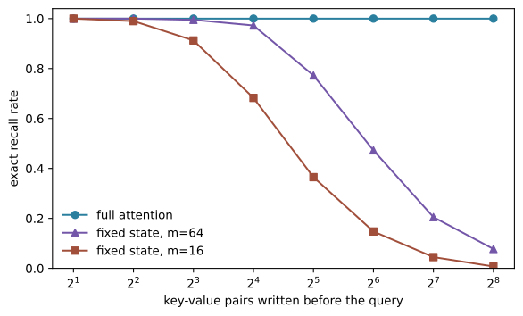
Real recurrent models are better than this raw memory: they distribute information across continuous dimensions, exploit structure, and learn selective forgetting, so they answer many tasks without exact token recall. The plot makes a bounded point — fixed state creates a capacity tradeoff, and more state improves it — not a benchmark ranking. For agents the distinction is operational. Summarizing a conversation’s intent is compression-friendly. Reproducing an exact identifier, a line of code, or a tool result from an arbitrary earlier position is associative recall. A workload of long streams with modest exact lookup can favor recurrence; a repository agent that must retrieve any of thousands of unique symbols wants periodic token-addressable attention, external retrieval, or both.
4.7 Hybrids and learned sparse attention
Because the two mechanisms fail differently, real long-context models interleave them. If L_f layers use full attention and L_r use fixed-state mixers, persistent state is a sum by layer type:
\operatorname{StateBytes}(T)=\operatorname{KVBytes}(L_f,T)+L_r\,P_{\text{state}}\,s, \tag{4.6}
where the first term is the Section 3.1 cache counting only the full-attention layers, and the second is the flat recurrent state. Only the full-attention layers carry a context-proportional slope. A cadence of three recurrent layers to one full-attention layer — the roughly 3:1 ratio now common in production — keeps a periodic exact-retrieval path while cutting the KV slope to about a quarter of an all-attention stack. The trap the equation guards against is real: do not apply an all-attention cache formula to every layer of a hybrid, and do not call a stack constant-memory just because most of its layers recur.
A third route keeps a full addressable history but computes only part of it. Sparse attention with fixed windows or blocks is cheap but encodes a predetermined visibility bias; learned selectors adapt to the query instead. Native Sparse Attention trains compression, selection, and a local branch end to end and co-designs the block structure for hardware (Yuan et al. 2025). Mixture of Block Attention applies the MoE idea to attention itself — a query routes to a selected set of key-value blocks — and can fall back to full attention (Lu et al. 2025). DeepSeek Sparse Attention uses a lightweight learned indexer to score past tokens and keep a fine-grained top-k for the main computation (DeepSeek-AI 2025). A one-line sketch of the MoBA idea — score blocks, keep the top few, attend only within them — shows the shape of the saving.
torch.manual_seed(1)
past = torch.randn(12, 8)              # 12 past tokens, width 8
query = torch.randn(8)
blocks = past.reshape(3, 4, 8)         # three blocks of four tokens
block_scores = (blocks.mean(1) @ query)         # score each block by its summary
keep = block_scores.topk(2).indices.tolist()    # attend to the best two blocks only
print("block scores:", [round(s, 2) for s in block_scores.tolist()], "-> keep blocks", sorted(keep))
block scores: [0.82, -1.91, 0.98] -> keep blocks [0, 2]The query keeps the two highest-scoring blocks and skips the third, so value mixing runs over 8 tokens instead of 12 — the same top-k gate as the router, now applied to regions of the sequence. Learned sparsity is not free: the selector must be trained with the backbone (a post-hoc mask changes the function the model learned), and an indexer that scores every past token still pays a linear search even as it saves the expensive value mixing. The three mechanisms form a design triangle — full attention (exact, growing state), fixed-state recurrence (bounded, lossy), learned sparse attention (addressable but selective, with index and miss-risk costs) — and hybrids place each where it earns its keep. No architecture label removes the need to measure recall, state, and runtime together.
4.8 Diffusion LMs and multi-token prediction
Everything so far kept the autoregressive contract: factor the sequence left to right, p(x_{1:T})=\prod_t p(x_t\mid x_{<t}), and commit one token at a time. Two research lines relax different parts of it, and both change decoding rather than the parameter or state ledgers. A diffusion language model corrupts tokens and learns to reverse the corruption over a block, refining many positions across several denoising steps; because positions can change before they are committed, it can revise and infill. A toy denoiser that reveals the highest-confidence positions of a target first makes the block-refinement shape concrete.
def block_denoise(target, steps=3, seed=1):
    """Toy diffusion decode: reveal highest-confidence positions over K steps."""
    torch.manual_seed(seed)
    slots = ["_"] * len(target)
    confidence = torch.rand(len(target))
    order = confidence.argsort(descending=True).tolist()
    per_step = -(-len(target) // steps)
    trace = []
    for s in range(steps):
        for position in order[s * per_step:(s + 1) * per_step]:
            slots[position] = target[position]
        trace.append("".join(slots))
    return trace


for i, snapshot in enumerate(block_denoise(list("MODEL"))):
    print(f"denoise step {i}: {snapshot}")
denoise step 0: M__E_
denoise step 1: MODE_
denoise step 2: MODELThe block fills in over three passes, several positions per step, rather than strictly left to right. “Multiple tokens in parallel” is not automatically faster: one step processes the whole block, and several steps may be needed, so latency depends on block size, step count, and kernel efficiency. Multi-token prediction (MTP) keeps the autoregressive trunk but adds heads that predict several future tokens during training, giving the shared representation denser supervision (Gloeckle et al. 2024). After training those heads can be discarded, or reused to propose tokens that the main model verifies — accepting only what it would have generated anyway.
def speculative_verify(draft, target_sequence):
    """Accept draft tokens until the first that the target would not have chosen."""
    accepted = []
    for token in draft:
        want = target_sequence[len(accepted)]
        accepted.append(want)
        if token != want:
            break            # mismatch: keep the correction, stop accepting
    return accepted


truth = "abcd"
print("draft 'abc':", "".join(speculative_verify("abc", truth)), "(3 accepted, all matched)")
print("draft 'axc':", "".join(speculative_verify("axc", truth)), "(1 accepted, then corrected)")
draft 'abc': abc (3 accepted, all matched)
draft 'axc': ab (1 accepted, then corrected)A draft that agrees advances several tokens for one verification pass; a draft that diverges is corrected at the first mismatch, so the output distribution is exactly the target’s. That is the durable comparison across all three schemes — dependency structure, not raw token counters. Autoregression commits one token; speculative MTP proposes several and verifies; diffusion refines a block over repeated passes. Their tokens-per-second numbers are not automatically comparable, and Chapter 10 owns the serving measurements that make them so.
4.9 Read the economics from config.json
Now the payoff: everything above lets us read a real model’s economics straight from its published config.json, without downloading weights. A config is not a full implementation, but it is usually enough to reject a bad capacity assumption. We embed three real configs — a dense model, an MoE, and a linear/full hybrid — as the exact field dicts a publisher ships.
# @save
REAL_CONFIGS = {
    "Llama 3.1 8B": {  # dense GQA -- https://huggingface.co/meta-llama/Llama-3.1-8B
        "model_type": "llama", "hidden_size": 4096, "intermediate_size": 14336,
        "num_hidden_layers": 32, "num_attention_heads": 32, "num_key_value_heads": 8,
        "head_dim": 128, "vocab_size": 128256, "tie_word_embeddings": False,
        "torch_dtype": "bfloat16", "_reported_total": 8_000_000_000, "_verified_on": "2026-07-19"},
    "DeepSeek-V3": {  # MoE + MLA -- https://huggingface.co/deepseek-ai/DeepSeek-V3-Base
        "model_type": "deepseek_v3", "hidden_size": 7168, "intermediate_size": 18432,
        "moe_intermediate_size": 2048, "num_hidden_layers": 61, "num_attention_heads": 128,
        "first_k_dense_replace": 3, "n_routed_experts": 256, "n_shared_experts": 1,
        "num_experts_per_tok": 8, "q_lora_rank": 1536, "kv_lora_rank": 512,
        "qk_nope_head_dim": 128, "qk_rope_head_dim": 64, "v_head_dim": 128,
        "vocab_size": 129280, "tie_word_embeddings": False, "torch_dtype": "bfloat16",
        "_reported_total": 671_000_000_000, "_verified_on": "2026-07-19"},
    "Qwen3-Next 80B-A3B": {  # 3:1 linear/full hybrid MoE -- https://huggingface.co/Qwen/Qwen3-Next-80B-A3B-Instruct
        "model_type": "qwen3_next", "hidden_size": 2048, "intermediate_size": 5120,
        "moe_intermediate_size": 512, "shared_expert_intermediate_size": 512,
        "num_hidden_layers": 48, "full_attention_interval": 4, "num_attention_heads": 16,
        "num_key_value_heads": 2, "head_dim": 256, "linear_num_key_heads": 16,
        "linear_num_value_heads": 32, "linear_key_head_dim": 128, "linear_value_head_dim": 128,
        "linear_conv_kernel_dim": 4, "num_experts": 512, "num_experts_per_tok": 10,
        "vocab_size": 151936, "tie_word_embeddings": False, "torch_dtype": "bfloat16",
        "_reported_total": 80_000_000_000, "_verified_on": "2026-07-19"},
}
The parser reads a config in leading-order matrix counts. It reuses one thing we refuse to reimplement: the canonical KV arithmetic from Section 3.1, loaded from Chapter 3’s tangled module so the whole book keeps a single cache formula. The per-architecture helpers below stay private; the public entry point is estimate_config.
# @save
import importlib.util
import sys
from dataclasses import dataclass
from pathlib import Path


def _load_ch03(name="ch03_kv_generated", relative="code/ch03/_generated.py"):
    bases = []
    try:  # inside the tangled module __file__ exists; during render it may not
        bases.append(Path(__file__).resolve().parents[2])
    except NameError:
        pass
    bases.append(Path.cwd())
    for base in bases:
        root = base
        for _ in range(6):
            candidate = root / relative
            if candidate.exists():
                spec = importlib.util.spec_from_file_location(name, candidate)
                module = importlib.util.module_from_spec(spec); sys.modules[name] = module
                spec.loader.exec_module(module); return module
            root = root.parent
    raise FileNotFoundError(relative)


_CH03 = _load_ch03()
KVConfig, kv_bytes = _CH03.KVConfig, _CH03.kv_bytes


def _dtype_bytes(cfg):
    return {"float32": 4, "float16": 2, "bfloat16": 2}[str(cfg.get("torch_dtype", "bfloat16"))]


def _embeddings(cfg):
    copies = 1 if cfg.get("tie_word_embeddings", False) else 2
    return copies * int(cfg["vocab_size"]) * int(cfg["hidden_size"])


def _gqa_params(cfg):
    w = int(cfg["hidden_size"]); qh = int(cfg["num_attention_heads"])
    kvh = int(cfg.get("num_key_value_heads", qh)); hd = int(cfg.get("head_dim", w // qh))
    return w * qh * hd + 2 * w * kvh * hd + qh * hd * w


def _mla_params(cfg):
    w = int(cfg["hidden_size"]); h = int(cfg["num_attention_heads"])
    nope, rope, val = (int(cfg[key]) for key in ("qk_nope_head_dim", "qk_rope_head_dim", "v_head_dim"))
    qr, kvr = int(cfg["q_lora_rank"]), int(cfg["kv_lora_rank"])
    return (w * qr + qr + qr * h * (nope + rope) + w * (kvr + rope)
            + kvr + kvr * h * (nope + val) + h * val * w)


def _linear_mixer(cfg):
    w = int(cfg["hidden_size"])
    key_dim = int(cfg["linear_num_key_heads"]) * int(cfg["linear_key_head_dim"])
    value_heads = int(cfg["linear_num_value_heads"]); value_dim = value_heads * int(cfg["linear_value_head_dim"])
    conv, kernel = 2 * key_dim + value_dim, int(cfg["linear_conv_kernel_dim"])
    params = (w * (2 * key_dim + 2 * value_dim) + w * (2 * value_heads) + conv * kernel
              + 2 * value_heads + int(cfg["linear_value_head_dim"]) + value_dim * w)
    fixed = value_heads * int(cfg["linear_value_head_dim"]) * int(cfg["linear_key_head_dim"]) + conv * (kernel - 1)
    return params, fixed
The three per-architecture estimators differ only in how they split the layers. The dense case counts GQA attention plus a SwiGLU MLP in every layer. The DeepSeek case counts MLA attention everywhere, a dense MLP in the first first_k_dense_replace layers, and E+S experts stored versus k+S active in the rest. The hybrid case counts full attention only every full_attention_interval layers and a linear mixer (with a flat recurrent state) in the others.
# @save
@dataclass(frozen=True)
class ArchitectureEstimate:
    """A model's reconstructed economics from its config fields alone.

    Bundles the two parameter ledgers of @sec-ch04-ledgers with the per-token
    and 32K-context sequence state, plus the error against the published total,
    so a spec can be sanity-checked before any weights are downloaded.

    Args:
        name: Model label.
        total: Reconstructed total parameters.
        active: Reconstructed active parameters per token.
        reported_total: The publisher's stated total.
        total_error_percent: Percent error of ``total`` against ``reported_total``.
        active_fraction: ``active / total``.
        kv_bytes_per_token: Cache bytes added per token by the attention layers.
        state_gib_32k: Persistent state at 32,768 tokens, batch 1, in GiB.
        fixed_state_bytes: Context-independent recurrent state (hybrids only).
    """

    name: str
    total: int
    active: int
    reported_total: int
    total_error_percent: float
    active_fraction: float
    kv_bytes_per_token: int
    state_gib_32k: float
    fixed_state_bytes: int


def estimate_config(name, cfg, context_tokens=32_768):
    """Reconstruct total and active parameters and sequence state from a config.

    Dispatches on ``model_type`` to the dense, MoE-plus-MLA, or linear/full
    hybrid estimator, counting the common trunk once and the experts by ledger,
    then sizes the KV cache with Chapter 3's ``kv_bytes`` over only the layers
    that actually keep a cache.

    Args:
        name: Model label carried into the result.
        cfg: The config field dict.
        context_tokens: Context length at which to price sequence state.

    Returns:
        An :class:`ArchitectureEstimate`.

    Raises:
        ValueError: If ``model_type`` is unsupported.
    """
    w, layers, mt = int(cfg["hidden_size"]), int(cfg["num_hidden_layers"]), cfg["model_type"]
    fixed = 0
    if mt == "llama":
        mlp = 3 * w * int(cfg["intermediate_size"])
        total = _embeddings(cfg) + layers * (_gqa_params(cfg) + mlp + 2 * w) + w
        active = total
        cache = KVConfig(name, layers, int(cfg["num_attention_heads"]),
                         int(cfg.get("head_dim", w // int(cfg["num_attention_heads"]))),
                         _dtype_bytes(cfg), kv_heads=int(cfg.get("num_key_value_heads", cfg["num_attention_heads"])))
    elif mt == "deepseek_v3":
        dense, moe = int(cfg["first_k_dense_replace"]), layers - int(cfg["first_k_dense_replace"])
        dense_mlp, expert_mlp = 3 * w * int(cfg["intermediate_size"]), 3 * w * int(cfg["moe_intermediate_size"])
        experts, selected, shared = int(cfg["n_routed_experts"]), int(cfg["num_experts_per_tok"]), int(cfg["n_shared_experts"])
        router = w * experts
        common = _embeddings(cfg) + layers * (_mla_params(cfg) + 2 * w) + dense * dense_mlp + w
        total = common + moe * ((experts + shared) * expert_mlp + router)
        active = common + moe * ((selected + shared) * expert_mlp + router)
        cache = KVConfig(name, layers, int(cfg["num_attention_heads"]), int(cfg["v_head_dim"]),
                         _dtype_bytes(cfg), latent_rank=int(cfg["kv_lora_rank"]), rope_key_dim=int(cfg["qk_rope_head_dim"]))
    elif mt == "qwen3_next":
        full = layers // int(cfg["full_attention_interval"]); linear = layers - full
        linear_params, fixed_scalars = _linear_mixer(cfg)
        experts, selected = int(cfg["num_experts"]), int(cfg["num_experts_per_tok"])
        expert_mlp, shared_mlp = 3 * w * int(cfg["moe_intermediate_size"]), 3 * w * int(cfg["shared_expert_intermediate_size"])
        router = w * experts
        common = (_embeddings(cfg) + full * _gqa_params(cfg) + linear * linear_params
                  + layers * (shared_mlp + router + 2 * w) + w)
        total, active = common + layers * experts * expert_mlp, common + layers * selected * expert_mlp
        cache = KVConfig(name, full, int(cfg["num_attention_heads"]), int(cfg["head_dim"]),
                         _dtype_bytes(cfg), kv_heads=int(cfg["num_key_value_heads"]))
        fixed = linear * fixed_scalars * _dtype_bytes(cfg)
    else:
        raise ValueError(f"unsupported model_type: {mt}")
    reported = int(cfg["_reported_total"])
    return ArchitectureEstimate(
        name, total, active, reported, 100 * (total - reported) / reported, active / total,
        kv_bytes(cache, 1), (kv_bytes(cache, context_tokens) + fixed) / 2**30, fixed)
We run the parser over all three configs and print the reconstruction.
for name, cfg in REAL_CONFIGS.items():
    e = estimate_config(name, cfg)
    print(f"{e.name:20s} total={e.total/1e9:8.3f}B  active={e.active/1e9:7.3f}B  "
          f"err={e.total_error_percent:+.3f}%  active_frac={e.active_fraction:5.2%}  "
          f"state@32k={e.state_gib_32k:.3f} GiB")
Llama 3.1 8B total= 8.030B active= 8.030B err=+0.378% active_frac=100.00% state@32k=4.000 GiB
DeepSeek-V3 total= 671.026B active= 37.552B err=+0.004% active_frac=5.60% state@32k=2.145 GiB
Qwen3-Next 80B-A3B total= 79.574B active= 3.774B err=-0.533% active_frac=4.74% state@32k=0.787 GiBThree published models, three total-count reconstructions within about half a percent, computed from a handful of integer fields. The stories the ledgers tell are exactly the two the chapter opened with. Llama’s active equals its total — a dense model has one ledger. DeepSeek-V3 stores 671B but activates only 37.6B (5.6%): MoE bends the active-weight curve, and its MLA cache holds the 32K state to 2.1 GiB. Qwen3-Next stores ~80B, activates ~3.8B, and its 3:1 linear/full hybrid bends the context-state curve — most layers keep only a flat recurrent state, so 32K tokens cost well under a gibibyte, though its periodic full-attention layers still contribute a context-proportional slice.
NoteIn the interview
Q. A model card says “3B active.” Your capacity plan assumes 3B of weights need to be resident. What’s wrong? Two things. First, “active” is a per-token compute count under the publisher’s convention — it usually excludes, or partially counts, embeddings, the output head, routers, shared experts, and norms; our parser puts Qwen3-Next’s active near 3.8B once those are included. Second, active parameters are not resident memory: every routed expert must be reachable, so the total (here ~80B) is what has to live somewhere in the serving topology, plus KV and recurrent state per sequence. The trap is multiplying total by k/E and sizing hardware to the result. The strong answer states the counting boundary and sizes both ledgers separately.
These reconstructions are dated evidence — configs change — so the embedded fields carry their source and a 2026-07-19 verification date; re-fetch each config.json before trusting a row in a real capacity decision.
4.10 Landscape 2026: the moving edge
NoteLandscape 2026 — very large capacity, low active fraction
The equations, the build, and the config-reading method above do not depend on which models are current; this box is the one dated snapshot and is safe to delete. As of the verification date, the visible open-weight trend is very large stored capacity with a low single-digit active fraction, and diversifying sequence mixers. Representative published figures (each from an official model card): DeepSeek-V4-Pro 1.6T total / 49B active and DeepSeek-V4-Flash 284B / 13B (hybrid compressed-sparse attention); Kimi K2.5 1T / 32B (384 experts, top-8 plus one shared, MLA); Qwen3.5 397B / 17B active (repeated groups of three Gated DeltaNet layers to one full-attention layer, 512 experts, top-10); GLM-5 744B / 40B (DeepSeek Sparse Attention); MiniMax-M2 230B / 10B, whose later guidance also documents full-attention variants — evidence that sparse attention is not a one-way migration; gpt-oss-120b 117B / 5.1B; and Llama 4 Maverick 400B / 17B (128 experts). Figure 4.7 plots them.
Settled enough to design around: conditional FFN computation as a capacity lever, compressed or shared KV for long context, and hybrid layer stacks as production architectures. Still contested: the best expert granularity and shared-expert design, auxiliary loss versus bias control, the ratio and placement of full attention, token- versus block-level learned sparsity, and whether diffusion decoding becomes a default.
Verify live: re-check each record against the current official model cards for DeepSeek-V4, Kimi K2.5, Qwen3.5, GLM-5, and successors before quoting any number. Verified: 2026-07-19.
Show the code that draws this figure
landscape = {
    "DeepSeek-V4-Pro": (1600, 49), "DeepSeek-V4-Flash": (284, 13), "Kimi K2.5": (1000, 32),
    "Qwen3.5": (397, 17), "GLM-5": (744, 40), "MiniMax-M2": (230, 10),
    "gpt-oss-120b": (117, 5.1), "Llama 4 Maverick": (400, 17),
}
fig, ax = plt.subplots(figsize=(6.6, 4.4))
xs = [t for t, _ in landscape.values()]
ax.scatter(xs, [a for _, a in landscape.values()], s=46, color="#2a7f9e", zorder=3)
for label, (t, a) in landscape.items():
    ax.annotate(label, (t, a), xytext=(4, 4), textcoords="offset points", fontsize=7.5)
lo, hi = min(xs) * 0.8, max(xs) * 1.2
ax.plot([lo, hi], [0.03 * lo, 0.03 * hi], "--", color="#7356a8", lw=1, label="3% active")
ax.plot([lo, hi], [0.05 * lo, 0.05 * hi], ":", color="#a14f3b", lw=1.2, label="5% active")
ax.set(xscale="log", yscale="log", xlabel="published total parameters (B)",
       ylabel="published active parameters (B)")
ax.legend(frameon=False, loc="lower right")
fig.tight_layout()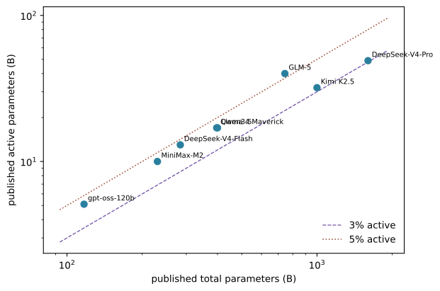
4.11 Summary
We pulled apart the two numbers a model card reports. MoE stores many experts and routes each token to a few, so stored capacity and active per-token compute become separate ledgers — and a low task loss can hide a collapsed router, so balance must be measured, not assumed. Linear-attention and state-space layers replace the growing KV cache with a fixed recurrent state, trading exact recall for bounded memory; hybrids interleave the two and sum state by layer type. We built a top-k router, a gated linear-attention block, and a config parser that reconstructed three real models to within half a percent. Chapter 10 turns these ledgers into serving decisions.
4.12 Exercises
Reconstruct a layer by hand. For width d={4096}, E={64} routed SwiGLU experts of width h_e={1024}, top-k={2}, and one shared expert, use Equation 4.3 to compute stored expert parameters, active expert parameters, and the active fraction. Check against the
stored/activecell. Then explain, in terms of the common trunk, why the model-wide active fraction differs from the expert-bank fraction.Sweep the balance coefficient. Extend
train_routerto also return the maximum per-expert load, then run balance weights of {0}, {0.01}, {0.1}, {0.5}, and {2}. Plot maximum load and accuracy against the coefficient. (a) Identify a range that prevents collapse without making balance the apparent task. (b) Explain why this coefficient cannot be transferred directly to a full language-model run.Price overflow policies. For N={8192}, E={32}, top-k={2}, and capacity factors {1.0}, {1.1}, and {1.25}, compute per-expert capacity. Construct a skewed load vector where one expert draws 30% of assignments and quantify dropped tokens at each factor. Discuss how rerouting and dropless dispatch each change correctness versus step-time risk.
Attach recall to the block.
associative_recall_curveuses an identity feature map. Modify it to route keys and values through aGatedLinearAttentionlayer’squery/valueprojections (decay pinned near 1) and re-measure at feature widths 16 and 64. Does the cliff move the same way? Explain which part of the change is the feature map and which is the state width.Widen the state, move the cliff. Using
associative_recall_curve, find for each of several feature widths the number of pairs at which recall first drops below 0.5. Plot that threshold against feature width. Is the relationship closer to linear or to something else, and how does that inform choosing a recurrent-state size for a target recall workload?Audit a new config. Add a fourth entry to
REAL_CONFIGSfor a current open-weight model not already present, writing a one-line field-semantics comment for each ambiguous field (for example whethernum_experts_per_tokincludes a shared expert). Runestimate_config, and where the total error exceeds two percent, name the omitted parameter family most likely responsible.