This is the infra round, and it is the one design where the product is the tokens: a platform that serves many teams’ models under service levels they can plan against. We run the seven moves from Chapter 33 on it, and the whole chapter is a single interview — prompt, scope, arithmetic, skeleton, dives, failure, and the one flipped requirement — for the model-infra family. The family’s identifying question is whether the product is tokens served under an SLO, and its fork, the one that sets every downstream choice, is strict per-request latency or throughput? The dominant bone is the model step itself, and the family’s signature numeric trap — sizing the KV cache from query heads instead of KV heads — lives right here, waiting to inflate the fleet fourfold. We compute the anchors live with the toolkit from Chapter 33 and Chapter 3’s KV calculator, and close with the family skeleton: the same bones re-instantiated across embedding, LoRA, and voice serving.
36.1 Scoping the platform
The interviewer opens with the underspecified version, the way they always do:
“A dozen product teams all want to call the open-weight models we host ourselves. Some power interactive chat, some run nightly batch jobs, some just need embeddings. Build the platform that serves all of them. It should be fast, it shouldn’t fall over when traffic spikes, and it should come out cheaper than the API vendor we’re leaving.”
Four clarifiers change the architecture; the rest only scale it. Do all teams share one model, or many? One shared 7B-class chat model plus one embedding model is a single fleet with continuous batching; a dozen fine-tuned variants is a multiplexing problem (LoRA multi-tenancy, Chapter 11) — I will assume the former and name the latter out of scope. Are the interactive, batch, and embedding workloads held to the same SLO? No, and that is the whole design: three tiers with three different promises, which forces workload isolation inside one fleet rather than one queue. When traffic spikes, do we serve the burst or shed it? This is the money question — buying peak capacity means idle silicon most of the day, shedding means someone’s request is refused — and I will design for autoscale-plus-shed, not over-provisioning. Why self-host at all? Cost and residency, which fixes the objective: dollars per GPU-hour over throughput, so every throughput lever becomes a cost lever.
The fork the interviewer will push on is the first tier’s: interactive is latency-bound, batch is throughput-bound, and the two want opposite batching policies on the same hardware. Naming that tension aloud in minute three is the senior signal; the rest of the hour resolves it. Restated with numbers, and with the non-goals said out loud, the requirements are Table 36.1.
Table 36.1: Requirements for the serving platform. Out of scope, stated aloud: per-team fine-tuned models (a multiplexing design), cross-region residency, and training capacity.
Tier
Workload
SLO
Load
Shape
Interactive
chat, RAG answers
p99 TTFT < 1 s; TPOT ~22 ms
~50 QPS peak, 3x bursts
4K context, 250-token cap
Batch
nightly summaries, tagging
best-effort, done by morning
~2M items/night
4K context, 300-token out
Embedding
index builds, semantic search
throughput target
on demand
512-token in, prefill only
36.2 The numbers first
Numbers before boxes. The model-infra anchors are KV memory per request, concurrency per device, the fleet a load implies, and the cost per token — and the first of these carries the trap. We recall Chapter 3’s KV equation (Equation 3.1) in one sentence — a request’s cache is layers times KV heads (not query heads) times head dimension times retained tokens times bytes, doubled for keys and values — and import its calculator rather than rebuild it.
KV, one 4K interactive request : 0.54 GB
KV, 16 concurrent              : 8.59 GB
the trap (32 query heads)      : 34.4 GB  -- 4x too high
Sixteen concurrent 4K requests hold 8.6 GB of cache; compute it from the thirty-two query heads and you get 34 GB and a fleet sized four times too large. The audible fix is one clause — “GQA caches eight KV heads, not thirty-two query heads” (Section 3.2) — and it is the single most reliable way to fail this round if you skip it. With the per-request number correct, capacity is a division: how many caches fit on a device, how long a request stays resident, and therefore how many devices a QPS number needs.
Show the code
per_device_mem = sd.kv_concurrency_per_device(hbm_bytes=80e9, weights_bytes=16e9, kv_bytes_per_request=per_req)batch_cap =32# interactive running-batch cap that holds TTFT (see the batching dive)ttft_ms, tpot_ms, out_cap =350.0, 22.0, 250residence_s = sd.completion_ms(ttft_ms, out_cap, tpot_ms) /1000in_flight = sd.concurrent_requests(qps=50, residence_seconds=residence_s)print(f"memory allows : {per_device_mem} requests/device (upper bound)")print(f"interactive residence : {residence_s:.1f} s (350 ms TTFT + 250 tok x 22 ms)")print(f"in flight at 50 QPS : {in_flight:.0f} requests (Little's law)")print(f"devices, memory-bound : {sd.devices_for_load(50, residence_s, per_device_mem)}")print(f"devices, batch-cap-bound : {sd.devices_for_load(50, residence_s, batch_cap)}")print(f"same under a 3x burst : {sd.devices_for_load(150, residence_s, batch_cap)}")
memory allows            : 104 requests/device (upper bound)
interactive residence    : 5.8 s  (350 ms TTFT + 250 tok x 22 ms)
in flight at 50 QPS      : 291 requests  (Little's law)
devices, memory-bound    : 4
devices, batch-cap-bound : 12
same under a 3x burst    : 36
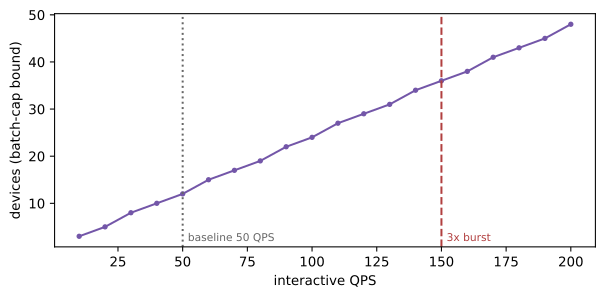
Two device numbers, and the gap between them is the design. Memory alone would fit about a hundred requests per card, which says four devices carry 50 QPS. But interactive TTFT will not survive a batch of a hundred — every request in the batch waits for the slowest — so we cap the running batch near 32 to hold the latency SLO, and that cap, not memory, binds: twelve devices at peak, thirty-six under a threefold burst. Which bound is active is the answer; the senior sentence is “memory says four, the TTFT batch cap says twelve, so I provision for twelve and the burst is a buy-or-shed decision, not a given.” The last anchor turns throughput into money, because self-hosting only pays if the arithmetic clears the vendor’s price.
Show the code
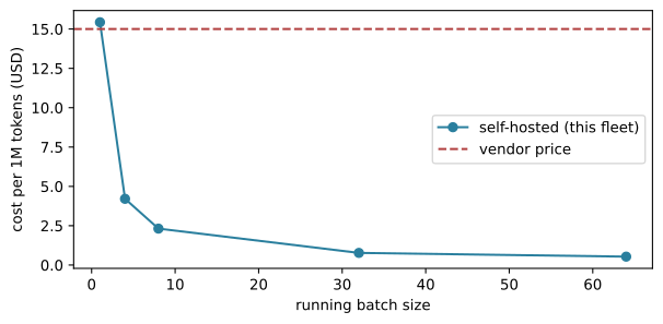
def cost_per_million(gpu_hour_price: float, throughput_tok_s: float) ->float:"""Dollars per million tokens = GPU-hour price over tokens served that hour."""return gpu_hour_price / (throughput_tok_s *3600) *1e6gpu_hour =2.50# illustrative on-demand dollars per GPU-hourvendor =15.00# illustrative vendor price, dollars per 1M output tokensfor b, thru in [(1, 45), (4, 165), (8, 300), (32, 900), (64, 1300)]:print(f"batch {b:2d}: {thru:4d} tok/s -> ${cost_per_million(gpu_hour, thru):5.2f} / 1M tokens")print(f"vendor reference : ${vendor:.2f} / 1M output tokens")
where P_{\text{GPU-hr}} is the device’s hourly price and \Theta is aggregate throughput in tokens per second. A single-stream device barely matches the vendor at $15 per million; batching past a handful of concurrent requests drops the same card below $1, a thirty-fold swing on identical silicon. So throughput is the cost lever, batching is the throughput lever, and batching is exactly what hurts interactive TTFT — Figure 36.1 draws the curve, and the tension it exposes is the rest of the chapter.
Show the code that draws this figure
import matplotlib.pyplot as pltpairs = [(1, 45), (4, 165), (8, 300), (32, 900), (64, 1300)]bs = [b for b, _ in pairs]costs = [cost_per_million(gpu_hour, t) for _, t in pairs]fig, ax = plt.subplots(figsize=(6.4, 3.2))ax.plot(bs, costs, marker="o", color="#2a7f9e", label="self-hosted (this fleet)")ax.axhline(vendor, ls="--", color="#b13f3f", label="vendor price")ax.set_xlabel("running batch size")ax.set_ylabel("cost per 1M tokens (USD)")ax.legend()fig.tight_layout()plt.show()
Figure 36.1: Why self-host? Cost per million tokens is dollars-per-GPU-hour over throughput, and throughput comes from batching: the same card swings from above the vendor line to a fraction of it. The catch is that every step right on this axis pushes interactive TTFT up.
NoteLandscape 2026 — the constants here are illustrative
The $2.50 GPU-hour price, the $15-per-million vendor reference, the 80 GB device, the 16 GB fp16 weights, the 22 ms TPOT, and the throughput-versus-batch numbers are teaching constants chosen for round arithmetic, not quotes. The KV formula and the cost formula do not move; the numbers move every hardware generation and pricing update. Verify live: check your accelerator’s datasheet, your measured TTFT/TPOT percentiles and decode throughput, and your provider’s current pricing before sizing a real fleet. Checked 2026-07-20.
36.3 The contract and the skeleton
The caller sees one inference API with a tier field and a stable model alias: interactive calls stream tokens and carry a hard output cap; batch calls submit-and-poll against a soft deadline; embedding calls return vectors with no decode phase. The service levels are per tier, and they are promises the platform owns, not the product teams: interactive p99 TTFT under one second and a published TPOT; batch best-effort with a morning deadline; embedding a throughput target. Under overload the gateway returns a retryable rejection to low-priority tiers rather than degrading everyone — abstention as a first-class response, at the fleet level. The success metrics are goodput (requests that met their SLO, not raw QPS), per-tier TTFT/TPOT percentiles, dollars per million tokens, and queue depth.
With the numbers and the contract fixed, most boxes are already chosen. Figure 36.2 is the model-infra skeleton: an admission gate, a batch scheduler that is the heart of the design, model runners holding paged KV, and a stream back — with a control plane that scales on queue depth and an observability plane watching the accelerator, not the host.
flowchart LR
    subgraph CP ["control plane"]
        AS["autoscaler<br/>queue depth + TTFT"]
        REG[("model registry<br/>weights · versions")]
    end
    Q["gateway / admission<br/>per-tier priority · quotas · load-shed"] --> TOK["tokenize"]
    TOK --> SCH["scheduler<br/>continuous batching<br/>per-tier queues"]
    SCH --> RUN["model runners<br/>prefill + decode · paged KV"]
    RUN --> DET["detokenize / stream"]
    DET --> LOG["log + meter<br/>goodput · TTFT/TPOT · $/tok"]
    AS -. scale .-> RUN
    REG -. load .-> RUN
Figure 36.2: Where does throughput come from without blowing interactive latency? The batch scheduler is the answer, and it sits behind an admission gate that can shed the batch tier to protect interactive p99.
Each box has one responsibility. The gateway authenticates the team, enforces per-tier quotas and rate limits, and is the only place that sheds load. The scheduler maintains per-tier queues and forms the running batch every step — this is where the latency-versus-throughput fork is resolved. The runners execute prefill and decode against paged KV so caches never fragment (Chapter 10 owns the engine; PagedAttention is the mechanism, Kwon et al. (2023)). The control plane scales the fleet on queue depth and streams weights from a versioned registry so a bad model rolls back by pointer flip. The observability plane meters the accelerator — utilization, batch size, KV occupancy, queue depth, per-tier percentiles — because host CPU tells you nothing about a GPU-bound system.
36.4 Deep dive: batching across mixed tiers
The interviewer forks here first, because this is the fork. The decision is continuous batching: the scheduler admits and retires requests at every decode step rather than freezing a batch until all its members finish (Yu et al. (2022); Chapter 10). Static batching wastes the fleet — a batch of a hundred waits for its one 250-token straggler while ninety-nine slots sit idle — and continuous batching is what turns the cost curve in Figure 36.1 from aspiration into throughput. But raw continuous batching optimizes throughput, and interactive TTFT is the opposite objective, which is why we run per-tier priority queues over one fleet: interactive requests preempt into the running batch under a size cap that bounds their queueing delay, and the batch tier is admitted only to fill the capacity interactive leaves. Figure 36.3 shows why the tiers even want different treatment — they load the two phases of one generation (Chapter 9) differently.
flowchart TD
    I["interactive tier<br/>p99 TTFT < 1s"] --> S{"scheduler<br/>priority + batch cap"}
    B["batch tier<br/>best-effort"] --> S
    E["embedding tier<br/>prefill only"] --> S
    S --> PF["prefill<br/>compute-bound, batches well"]
    PF --> DC["decode<br/>bandwidth-bound, sets TPOT"]
    DC --> O["stream tokens"]
    PF --> V["return vector<br/>no decode"]
Figure 36.3: Which phase do I optimize for which SLO? Prefill is compute-bound and batches cheaply; decode is memory-bandwidth-bound and owns the per-token latency an interactive user feels. Embeddings are prefill only.
The alternative is separate fleets per tier: clean isolation, but each fleet is provisioned for its own peak and idle the rest of the day, which throws away the cost win we came for. The middle path — one fleet, priority scheduling — buys most of the isolation at a fraction of the idle cost, and the residual risk is starvation, which the failure pass handles. When the interviewer pushes — “what stops a flood of batch work from starving interactive?” — the answer is three-part: batch requests are preemptible by contract, the scheduler reserves headroom for the interactive tier, and admission sheds batch before interactive ever queues. The batch cap is not a magic number; it is set by the measured TTFT-versus-batch curve for this model on this device, and it is the single knob the SLO negotiation turns.
36.5 Deep dive: memory, the KV trap, and quantization
Serving capacity is a memory statement before it is a compute statement, which is why the KV trap from Section 36.2 is not a footnote — it sets how many requests a device holds, and therefore the fleet size and the cost. Paged KV (the runner’s allocator) keeps that memory from fragmenting so the concurrency the arithmetic predicts is the concurrency you actually get. The lever that buys more of it is quantization: serving weights and KV at FP8 or INT4 frees HBM for more concurrent caches and lowers dollars per token on both axes at once (Chapter 10 owns the method). The decision is to quantize the shared serving weights once the quality gate clears, and to keep an fp16 fallback path.
The alternative — never quantize, stay fp16 — is the safe default that leaves half the concurrency and much of the cost win on the table. When the interviewer pushes — “how do you know it’s safe?” — the answer is the discipline that separates a serving platform from a demo: quantization is a validation problem, not a performance setting. Every team’s traffic is a different distribution, so the quantized build must pass each team’s own eval set (Chapter 22’s calibrated gates) before it serves their traffic, and a quiet quality regression on one team’s workload is a rollback, not a tuning note. The trap and this dive are the same lesson from two directions: the model step’s memory is the design’s binding constraint, and both the arithmetic and the quantization gate exist to respect it honestly.
36.6 Deep dive: autoscaling on queue depth
The last fork is the control signal, and the common wrong answer is “GPU utilization, like any web service.” A decode fleet is memory-bandwidth-bound, so it can sit at modest FLOP utilization while latency is already blown — bandwidth is saturated, not compute — and utilization lags the thing the user feels. The decision is to autoscale on queue depth and TTFT-SLO headroom, the leading indicators of the promise we actually made. Figure 36.4 draws the loop: rising queue depth adds a warm runner, a draining queue scales the batch pool toward zero, and when the SLO is at risk faster than scaling can respond, admission sheds the batch tier first.
flowchart LR
    M["metrics<br/>queue depth · KV occupancy<br/>TTFT/TPOT per tier · GPU util"] --> A{"autoscaler"}
    A -->|"queue rising"| UP["add warm runner"]
    A -->|"queue draining"| DOWN["scale batch pool to zero"]
    M --> SH{"admission"}
    SH -->|"SLO at risk"| SHED["shed batch tier first"]
Figure 36.4: Queue depth rising while GPU utilization stays flat means scheduler- or memory-bound, not compute-bound. Which signal does the control plane trust? The one tied to the SLO, not the one tied to the silicon.
The alternative, scaling on GPU or CPU utilization, is what most infra teams reach for and what mis-serves this workload; naming why it fails is the senior move. When the interviewer pushes on cold starts — a new runner loads 16 GB of weights before it serves anything, and that load time is an SLO miss — the answer is a warm pool sized to the burst you promise to absorb, plus scale-to-zero for the spiky batch tier where cold start is free. The warm pool is not waste; it is the price of the burst SLO, and quoting that price (idle devices times the GPU-hour rate) against the cost of shedding is exactly the buy-or-shed decision the anchors set up. Figure 36.5 makes it visible.
Figure 36.5: Buy the burst or shed it? Devices needed rise linearly with interactive QPS at the batch-cap-bound concurrency. Provisioning for the dotted baseline and shedding above it is cheap; provisioning for the dashed 3x burst means most cards sit idle most of the day.
36.7 Tradeoffs, failure, and cost as an attack
Every lever above trades something, and the tradeoff table (Table 36.2) is the failure pass in compressed form: choice, what it costs, what it buys, the residual risk, and the control that holds the risk.
Table 36.2: The serving platform’s decisions, costed.
Choice
Cost
Buys
Risk
Control
Continuous batching
per-request queueing latency
large throughput / cost win
interactive TTFT hit
cap interactive batch; per-tier priority
Quantization (FP8/INT4)
quality delta
more concurrent KV, cheaper per token
silent quality regression
gate on each team’s eval set; fp16 fallback
Load-shed on overload
rejected low-priority work
protects interactive p99
dropped batch jobs
downgrade the tier, don’t degrade all; 429 + retry
Prefill/decode disaggregation
added hops, network transfer
long prompts stop stalling decode
infra complexity
adopt only at scale; chunked prefill first
The failure modes follow the same order. Under a burst that outruns the warm pool, the queue explodes and TTFT violates first; the control is to shed the batch tier and hold interactive, degrading one tier rather than all. A batch job that floods the shared fleet starves interactive; the control is priority plus reserved headroom plus preemption, and the pager fires only if interactive p99 stays violated after shedding. KV exhaustion under an under-provisioned fleet forces preemption-and-recompute or rejection, never silent corruption. A bad model version is caught by canary and rolled back by alias flip, because the registry made the deployable unit a versioned pointer.
Cost is an attack surface here in a way the vendor never exposed us to. Since dollars scale as throughput over price, an adversary who sends adversarially long contexts or floods max-output requests is buying capacity we pay for — a denial-of-wallet and a denial-of-service at once (Chapter 26 develops the framing). The controls are the caps we already put in the contract: a hard context ceiling, the output cap, per-team rate limits, and admission control that treats an anomalous cost spike as an incident. And because the fleet is multi-tenant, one team’s traffic can degrade another’s; per-tier and per-team quotas are the isolation boundary, and a quota breach pages before it becomes a shared-fleet outage.
36.8 Evolution: when prompts get long
Build order follows the evidence. Ship one model, one fleet, continuous batching, and the interactive tier alone; measure TTFT, TPOT, and goodput before adding anything, because those curves set every later knob. Add the batch tier with priority scheduling once interactive is stable. Add quantization when a team’s eval gate clears it. Add autoscaling when the traffic histogram — not a guess — justifies the warm pool. Disaggregation waits until scale demands it.
Then the interviewer flips one requirement: “a team now needs 128K-context requests.” The delta is sharp and mostly numeric. KV per request scales with retained tokens, so it jumps from half a gigabyte to roughly sixteen, and per-device concurrency collapses from about a hundred to a handful — the anchor arithmetic from Section 36.2, rerun with tokens=131_072, is the whole answer to “how much does this change the fleet.” Prefill now dominates, and a long prompt monopolizes a runner long enough to stall every decode sharing it, which is precisely the condition prefill/decode disaggregation exists for: split prefill and decode onto separate pools so a giant prompt fills a prefill card without freezing anyone’s token stream (Zhong et al. (2024); Patel et al. (2024)). What survives is almost everything — the contract, the batching policy for the short tiers, the autoscaling signal, and the cost formula are untouched; only the long-context tier gets a disaggregated path, and chunked prefill is the cheaper first step before the full split. Naming what changes and what survives in two sentences is the finish line.
36.9 Probes and the family skeleton
“Queue depth is climbing but GPU utilization is flat at 60%. What’s happening?” The fleet is memory- or scheduler-bound, not compute-bound: you cannot batch more because KV cache is full or the batch cap is holding, so requests queue while the FLOPs sit idle. The fix is not more compute — it is more KV headroom (quantize, evict, raise the cap if TTFT allows), and the trace shows it as rising queue depth with flat utilization and climbing KV occupancy. Adding cards helps only because it adds HBM, not because it adds compute.
“Why not autoscale on GPU utilization like everything else?” Because a decode fleet is bandwidth-bound: it can be at moderate utilization while TPOT is already over budget, so utilization is a lagging, misleading proxy for the promise you made. Scale on the leading indicators tied to the SLO — queue depth and TTFT headroom — and keep utilization as a cost metric, not a scaling trigger.
“A batch job just tanked interactive latency. Prevent it.” Per-tier priority with reserved interactive headroom, batch requests preemptible by contract, and admission that sheds batch before interactive queues. The shared fleet is the cost win; the priority scheduler and quotas are what make sharing safe.
The model-infra skeleton — admission, a batch scheduler, paged-KV runners, autoscale on queue depth — re-instantiates across the family with one constraint changed and one decision flipped (Table 36.3).
Table 36.3: The model-infra family: same bones, one changed constraint, one flipped decision.
tiny max-batch, streaming/speculative decode, latency over throughput, no batch tier
The embedding sibling is the sharpest tell that you understood the fork: strip the decode phase and the KV trap vanishes, the latency-versus-throughput tension disappears, and the design collapses to throughput-first static batching — a different answer produced by the same procedure.
36.10 Summary
The model-infra round is an argument about accelerator memory and batching, run under per-tier SLOs. We scoped a multi-team serving platform, split it into interactive, batch, and embedding tiers, and computed the anchors live: KV per request (with the query-heads trap that inflates the fleet fourfold), concurrency per device, the fleet a QPS number implies, and cost as dollars-per-GPU-hour over throughput. The skeleton is an admission gate, a continuous-batching scheduler with per-tier priority, paged-KV runners, and autoscaling on queue depth — not utilization. Batching, quantization, load-shed, and disaggregation are the costed decisions; cost itself is an attack surface. Chapter 37 turns to measurement infra: an eval platform.
36.11 Exercises
Resize for a bigger model. Swap the 7B-class model for a 70B-class one that needs two devices under tensor parallelism. Rebuild the KV config, recompute per-device concurrency (the weights now split across two cards), and report which anchor number moves most and why the fleet math changes shape.
Flip the mix. The interviewer says the platform is now 80% batch, 20% interactive. Redraw only the boxes in Figure 36.2 that change, and re-argue the batching policy and the autoscaling signal for the new dominant tier.
Find the break-even (multi-part). Using the cost cell: (a) find the smallest running batch size at which self-hosting beats the $15-per-million vendor line; (b) drop the GPU-hour price to $1.20 and recompute that batch; (c) at a fixed batch of 8, find the vendor price below which self-hosting stops paying.
Work the trap both ways. Recompute the sixteen-request KV number using query heads, state the ratio to the correct number, and explain in one sentence why GQA caches only the KV heads (recall Section 3.2). Then switch the config to MQA (one KV head) and report the new per-device concurrency.
Buy or shed (multi-part). Recompute the fleet under a 4x burst. Then instead of buying capacity, cut the interactive output cap from 250 to 100 tokens, recompute residence via completion_ms and the fleet again, and state which knob you would pull first and what it costs the user.
Size the embedding tier. Two million embeddings a night, 512-token inputs, prefill only. Estimate the throughput it needs, argue whether it shares the interactive fleet or gets its own pool, and name the one anchor from Section 36.2 that does not apply to a prefill-only workload.
Run the long-context flip. Recompute per_req and per-device concurrency at tokens=131_072, name the single architectural change from Table 36.2 you would make, and list the boxes in the skeleton that survive the flip unchanged.
Kwon, Woosuk et al. 2023. “Efficient Memory Management for Large Language Model Serving with PagedAttention.”Proceedings of the ACM SIGOPS Symposium on Operating Systems Principles.
Patel, Pratyush, Esha Choukse, Chaojie Zhang, et al. 2024. “Splitwise: Efficient Generative LLM Inference Using Phase Splitting.”2024 ACM/IEEE 51st Annual International Symposium on Computer Architecture (ISCA), 118–32.
Yu, Gyeong-In, Joo Seong Jeong, Geon-Woo Kim, Soojeong Kim, and Byung-Gon Chun. 2022. “Orca: A Distributed Serving System for Transformer-Based Generative Models.”16th USENIX Symposium on Operating Systems Design and Implementation (OSDI 22), 521–38.
Zhong, Yinmin, Shengyu Liu, Junda Chen, et al. 2024. “DistServe: Disaggregating Prefill and Decoding for Goodput-Optimized Large Language Model Serving.”18th USENIX Symposium on Operating Systems Design and Implementation (OSDI 24), 193–210.