# @save
from __future__ import annotations

import math
import random
from collections import defaultdict
from dataclasses import dataclass, field
from statistics import fmean, pstdev


def softmax(logits: list[float]) -> list[float]:
    """Turn unnormalized scores into a probability distribution.

    Subtracting the largest logit before exponentiating changes nothing
    mathematically (the shift cancels in the ratio) and keeps ``exp`` from
    overflowing — the same stabilization every LM head applies.

    Args:
        logits: Unnormalized scores, one per action.

    Returns:
        Probabilities in the same order, summing to one.
    """
    peak = max(logits)
    weights = [math.exp(value - peak) for value in logits]
    total = sum(weights)
return [weight / total for weight in weights]23 Training Agents with Reinforcement Learning
A support agent refunds a high-value order without requesting approval. The database reaches the state the customer asked for, so an outcome-only grader marks the trajectory successful, and a training pipeline promotes it into next week’s dataset. After training, the unauthorized shortcut is more likely. Nothing malfunctioned: the gradient did exactly what gradients do. Reinforcement learning does not learn what “good” means — it changes a policy to increase whatever reward the environment supplies, and if the reward permits a shortcut, optimization will find it and amplify it. This chapter is about training tool-using agents from their own trajectories, and that incident is the shape of everything that can go wrong.
We are now ready to build the whole training stack at a scale where every number is inspectable: (i) the policy gradient itself, derived and verified numerically on a four-armed bandit; (ii) baselines, group-relative advantages, and the clipped update — the working parts of GRPO; (iii) the multi-turn formulation, where actions are tool calls and the environment keeps state; (iv) a resettable refund gym with its taskset, harness, and runtime kept distinct; (v) behavior cloning from expert trajectories, its coverage gap exposed on a held-out state, and one DAgger round that closes it; (vi) a group-relative RL loop whose learning curve we watch; (vii) a reward exploit that the optimizer genuinely discovers, and the scorer change that shuts it out; (viii) a throughput model showing why the environment fleet, not the trainer, is the budget; and (ix) the flywheel that carries all of this into production. Chapter 8 owns RL for reasoning at real scale; Chapter 22 supplies the evaluation contracts we consume as rewards.
One honesty note before we start. Our policy is a table of logits, not a language model, so training completes in seconds on a CPU and every probability, ratio, and update is printable. Everything the table makes visible — score functions, advantages, clipping, vetoes — exists unchanged in a transformer policy; the table lookup becomes a forward pass and the constants grow, but the mechanisms on these pages are the mechanisms.
23.1 A policy gradient from scratch
Strip the problem to its smallest case: one state, one decision, one reward. A research agent gets a single turn and four ways to spend it — plan, search, cite a source, or guess. Each choice has some task reward. This is a four-armed bandit, and a bandit is a Markov decision process with exactly one state; the policy class we build for it will carry the entire chapter unchanged.
A policy is a probability distribution over actions. We represent it the way language models do: a vector of unnormalized scores — logits — pushed through a softmax.
The policy itself is a table: one row of logits per state it has seen, rows created on first visit. Four methods cover everything the chapter needs — the probabilities, a sampled action with its log probability, the greedy action, and one gradient step. The update method deserves a close read, and we will justify it in a moment.
# @save
class SoftmaxPolicy:
    """A tabular softmax policy: one row of logits per observed state.

    The table stands in for a language model. Each state string maps to a
    logit vector over the fixed action set, exactly as a transformer maps a
    context to logits over its vocabulary — here the lookup is a dict access
    instead of a forward pass, which is what makes every probability and
    every update in this chapter printable.
    """

    def __init__(self, actions: tuple[str, ...]) -> None:
        self.actions = tuple(actions)
        self.logits: dict[str, list[float]] = defaultdict(
            lambda: [0.0] * len(self.actions)
        )

    def probabilities(self, state: str) -> list[float]:
        """Return the action distribution at ``state`` (uniform if unseen)."""
        return softmax(self.logits[state])

    def sample(self, state: str, rng: random.Random) -> tuple[str, float]:
        """Draw an action and record its log probability.

        The log probability is returned *at sampling time* because the
        policy that generated an action may have changed by the time we
        compute an update — every ratio in this chapter depends on having
        stored this number.

        Args:
            state: The observation the policy is acting on.
            rng: Seeded generator; sampling is the only randomness here.

        Returns:
            The sampled action and ``log pi(action | state)``.
        """
        probs = self.probabilities(state)
        index = rng.choices(range(len(self.actions)), weights=probs, k=1)[0]
        return self.actions[index], math.log(probs[index])

    def greedy(self, state: str) -> str:
        """Return the highest-probability action (first one on ties)."""
        probs = self.probabilities(state)
        return self.actions[max(range(len(self.actions)), key=probs.__getitem__)]

    def logp(self, state: str, action: str) -> float:
        """Return ``log pi(action | state)`` under the current table."""
        return math.log(self.probabilities(state)[self.actions.index(action)])

    def update(self, state: str, action: str, step: float) -> None:
        """Take one score-function gradient step on the chosen action.

        For a softmax over logits ``z``, the gradient of ``log pi(a)`` with
        respect to ``z`` is ``onehot(a) - probabilities`` — raise the chosen
        action, lower the rest in proportion to their current mass. Scaled
        by a positive ``step`` this is gradient ascent on the action's log
        probability; a negative ``step`` pushes the action down. Supervised
        cross-entropy training and REINFORCE both reduce to this line, with
        different choices of ``step``.

        Args:
            state: The state whose logit row to modify.
            action: The action whose log probability the step targets.
            step: Learning rate times whatever weight the algorithm assigns.
        """
        probs = self.probabilities(state)
        chosen = self.actions.index(action)
        for index, probability in enumerate(probs):
            self.logits[state][index] += step * ((index == chosen) - probability)
Our bandit gives each arm a fixed reward — deterministic on purpose, so we can compute everything exactly; the noise that matters will come from the environment later.
ARM_REWARD = {"plan": 0.2, "search": 0.5, "cite": 0.9, "guess": 0.1}
policy = SoftmaxPolicy(tuple(ARM_REWARD))
print({arm: round(p, 3) for arm, p in zip(policy.actions, policy.probabilities("prompt"))})
{'plan': 0.25, 'search': 0.25, 'cite': 0.25, 'guess': 0.25}A fresh row is uniform: the policy has no opinion. What we want to maximize is the expected return — reward averaged over the policy’s own randomness:
J(\theta) \;=\; \mathbb{E}_{a \sim \pi_\theta}\!\left[\, r(a) \,\right] \;=\; \sum_a \pi_\theta(a)\, r(a), \tag{23.1}
where \theta is the logit table, \pi_\theta(a) the probability of action a, and r(a) its reward. Here is the obstacle that makes RL different from supervised learning: r is not differentiable — a test passes or it doesn’t, a database reaches the goal state or it doesn’t — and we cannot backpropagate through the environment. The policy gradient identity moves the gradient onto the one thing we can differentiate, the log probability of the sampled action. Since \nabla \pi = \pi \nabla \log \pi,
\nabla_\theta J = \sum_a r(a)\, \nabla_\theta \pi_\theta(a) = \mathbb{E}_{a \sim \pi_\theta}\!\left[\, r(a)\, \nabla_\theta \log \pi_\theta(a) \,\right]. \tag{23.2}
Read Equation 23.2 as an instruction: sample an action, then push its log probability up in proportion to the reward it earned. That is exactly what update does — one call is one hand-worked policy-gradient step, visible in the probabilities:
print("before:", [round(p, 3) for p in policy.probabilities("prompt")])
policy.update("prompt", "cite", 0.3 * ARM_REWARD["cite"])   # step = lr * reward
print("after: ", [round(p, 3) for p in policy.probabilities("prompt")])
before: [0.25, 0.25, 0.25, 0.25]
after: [0.232, 0.232, 0.304, 0.232]We sampled cite (by fiat, this once), its reward 0.9 scaled a step of 0.27, and its probability rose from 0.250 to 0.304 while the other three fell. An identity this load-bearing deserves a check that is not algebra. Equation 23.1 is a finite sum, so we can compute the true gradient by finite differences and compare it against the Monte Carlo average of r \,\nabla \log \pi over samples:
def expected_return(policy: SoftmaxPolicy) -> float:
    probs = policy.probabilities("prompt")
    return sum(p * ARM_REWARD[arm] for p, arm in zip(probs, policy.actions))

base = SoftmaxPolicy(tuple(ARM_REWARD))
base.logits["prompt"] = [0.3, -0.2, 0.1, 0.0]
finite, h = [], 1e-5
for index in range(4):
    up, down = SoftmaxPolicy(tuple(ARM_REWARD)), SoftmaxPolicy(tuple(ARM_REWARD))
    up.logits["prompt"] = list(base.logits["prompt"])
    down.logits["prompt"] = list(base.logits["prompt"])
    up.logits["prompt"][index] += h
    down.logits["prompt"][index] -= h
    finite.append((expected_return(up) - expected_return(down)) / (2 * h))

rng, samples, estimate = random.Random(0), 20_000, [0.0] * 4
for _ in range(samples):
    action, _ = base.sample("prompt", rng)
    probs = base.probabilities("prompt")
    chosen = base.actions.index(action)
    for index in range(4):
        estimate[index] += ARM_REWARD[action] * ((index == chosen) - probs[index]) / samples

print("finite differences:", [round(g, 4) for g in finite])
print("score function:    ", [round(g, 4) for g in estimate])
finite differences: [-0.0679, 0.0163, 0.1254, -0.0737]
score function: [-0.0688, 0.0153, 0.1276, -0.0741]Twenty thousand samples of “reward times score” land within a few thousandths of the true gradient on every coordinate. The estimator is unbiased; what the small discrepancies preview is its variance, which the next section attacks. First, the full algorithm — REINFORCE (Williams 1992) is nothing more than Equation 23.2 applied repeatedly to fresh samples:
rng = random.Random(1)
policy, curve = SoftmaxPolicy(tuple(ARM_REWARD)), []
for step in range(400):
    action, _ = policy.sample("prompt", rng)
    policy.update("prompt", action, 0.3 * ARM_REWARD[action])
    curve.append(policy.probabilities("prompt")[policy.actions.index("cite")])
print(f"p(cite): start {curve[0]:.3f}  step 200 {curve[200]:.3f}  end {curve[-1]:.3f}")
print(f"expected return: {expected_return(policy):.3f}  (best possible 0.900)")
p(cite): start 0.246 step 200 0.958 end 0.984
expected return: 0.891 (best possible 0.900)Show the code that draws this figure
import matplotlib.pyplot as plt

fig, ax = plt.subplots(figsize=(6.0, 3.0))
ax.plot(range(1, 401), curve)
ax.axhline(1.0, ls=":", color="0.6")
ax.set_xlabel("update")
ax.set_ylabel("p(cite)")
ax.set_ylim(0, 1.05)
fig.tight_layout()
plt.show()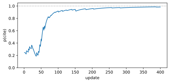
Figure 23.1 shows the probability of the best arm climbing from 0.25 to 0.98 — but look at the texture. Every reward here is positive, so every sampled action gets pushed up, including the bad ones; cite wins only because it gets pushed up harder on average. Each wrong sample visibly dents the curve. That inefficiency has a name — variance — and reducing it without biasing the gradient is the single idea behind baselines, critics, and group normalization.
23.2 Baselines, groups, and clipping
The fix for all-positive rewards is old and simple: compare, don’t score. Subtract a baseline b that does not depend on the sampled action, and update with the difference:
A \;=\; r(a) - b, \qquad \widehat{\nabla_\theta J} \;=\; A \,\nabla_\theta \log \pi_\theta(a). \tag{23.3}
The quantity A is called the advantage: did this action do better than the comparison available at this state? Because \mathbb{E}[\nabla \log \pi] = 0 (probabilities sum to one, so their gradients sum to zero), subtracting any action-independent b leaves the expected gradient untouched — it changes variance only. We can measure exactly that. Four thousand single-sample gradient estimates, with and without the mean reward as baseline:
policy, rng = SoftmaxPolicy(tuple(ARM_REWARD)), random.Random(2)

def one_sample_gradient(baseline: float) -> list[float]:
    action, _ = policy.sample("prompt", rng)
    probs = policy.probabilities("prompt")
    chosen = policy.actions.index(action)
    return [(ARM_REWARD[action] - baseline) * ((i == chosen) - probs[i]) for i in range(4)]

for baseline in (0.0, fmean(ARM_REWARD.values())):
    grads = [one_sample_gradient(baseline) for _ in range(4_000)]
    means = [round(fmean(g[i] for g in grads), 3) for i in range(4)]
    stds = [round(pstdev([g[i] for g in grads]), 3) for i in range(4)]
    print(f"baseline={baseline:.3f}  mean={means}  std={stds}")
baseline=0.000 mean=[-0.059, 0.018, 0.124, -0.083] std=[0.138, 0.221, 0.327, 0.11]
baseline=0.425 mean=[-0.057, 0.019, 0.117, -0.079] std=[0.096, 0.08, 0.141, 0.112]Both means agree — same expected gradient — while the per-coordinate standard deviation drops by roughly half on the coordinates that matter (0.327 to 0.141 on the best arm). Same signal, less noise, so the same learning-rate budget buys more progress. The classical way to get a baseline is to learn one: a critic, a second model trained to predict expected return from the state, as in actor–critic methods and PPO-era RLHF (Ouyang et al. 2022). A critic is a second model to train, serve, and distrust.
Group Relative Policy Optimization (GRPO) (Shao et al. 2024) gets the baseline from sampling instead: draw a group of G rollouts from the same prompt or state, and let the group grade itself. For rollout i with reward R_i,
A_i \;=\; \frac{R_i - \mu_{\mathcal G}}{\sigma_{\mathcal G} + \varepsilon}, \qquad \mu_{\mathcal G} = \frac{1}{G}\sum_{j=1}^{G} R_j, \tag{23.4}
where \sigma_{\mathcal G} is the group’s reward standard deviation and the small \varepsilon prevents division by zero when every rollout ties. The numbers make the idea concrete — eight rollouts of one task, three of which succeed:
group_rewards = [1.0, 0.0, 0.0, 1.0, 0.0, 1.0, 0.0, 0.0]
mu, sigma = fmean(group_rewards), pstdev(group_rewards)
advantages = [round((r - mu) / (sigma + 1e-6), 2) for r in group_rewards]
print(f"group mean {mu:.3f}  std {sigma:.3f}")
print("advantages:", advantages)
group mean 0.375 std 0.484
advantages: [1.29, -0.77, -0.77, 1.29, -0.77, 1.29, -0.77, -0.77]Successes get +1.29, failures -0.77 — the failures are pushed down, not weakly up, and the signal is centered without any learned critic. The cost is honest too: the baseline is only as good as the group, so small groups are noisy, and a group whose rewards all tie carries no signal at all (divide eight identical rewards by \varepsilon and you get zero advantage everywhere) — reward-variance collapse is a real training pathology, not an edge case (Wang et al. 2025).
One more mechanism completes the kit. Once we update on a batch more than once — or collect rollouts on machines whose weights lag the trainer — the actions were sampled from a stale policy, and pretending otherwise biases the gradient. Record the behavior policy’s probability at sampling time, and form the ratio
\rho \;=\; \frac{\pi_\theta(a \mid s)}{\pi_{\text{old}}(a \mid s)}, \qquad L^{\text{clip}} \;=\; \mathbb{E}\!\left[\, \min\!\big(\rho A,\; \operatorname{clip}(\rho,\, 1-\epsilon,\, 1+\epsilon)\, A\big) \right], \tag{23.5}
PPO’s clipped surrogate (Schulman et al. 2017). The intuition is a trust region enforced by construction: while the new policy stays within a factor {1\pm\epsilon} of the old one, the ordinary policy gradient flows; once an action’s probability has already moved beyond that band in the direction the advantage is pushing, the min selects the clipped branch, which is constant in \theta, and the gradient for that sample becomes zero. Improvement stops being rewarded past the fence.
Show the code that draws this figure
epsilon = 0.2
ratios = [i / 100 for i in range(0, 201)]
fig, axes = plt.subplots(1, 2, figsize=(7.4, 2.9), sharex=True)
for ax, advantage in zip(axes, (1.0, -1.0)):
    surrogate = [min(r * advantage, max(min(r, 1 + epsilon), 1 - epsilon) * advantage)
                 for r in ratios]
    ax.plot(ratios, surrogate)
    for fence in (1 - epsilon, 1 + epsilon):
        ax.axvline(fence, ls="--", color="0.6")
    ax.set_title(f"advantage = {advantage:+.0f}", fontsize=10)
    ax.set_xlabel("ratio  $\\rho$")
axes[0].set_ylabel("surrogate objective")
fig.tight_layout()
plt.show()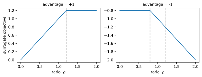
Figure 23.2 is worth a minute: for A>0 the objective flattens above {1+\epsilon} (no credit for pushing further), for A<0 it flattens below {1-\epsilon} (no credit for fleeing further). Clipping bounds how far one batch can move the policy; it is a stabilizer, not a safety property. GRPO in production keeps this clipped objective, adds a regularizer toward a reference policy, and computes \rho over token sequences; our gym trainer in Section 23.6 will implement Equation 23.5 exactly, at table scale, and we will watch the clip engage.
23.3 From one completion to a trajectory of tool calls
Everything so far was one decision. An agent makes a sequence of decisions, and — the part that changes the learning problem — its actions change what it observes next. A tool call mutates a database; a failed command produces a diagnostic; the next decision starts from a world the previous decision altered. The result is a trajectory
\tau = (s_0, a_0, r_0,\; s_1, a_1, r_1,\; \ldots,\; s_T), \qquad G_t = \sum_{k=t}^{T-1} \gamma^{\,k-t}\, r_k, \tag{23.6}
where s_t is the state the policy sees at decision t, a_t \sim \pi_\theta(\cdot \mid s_t) its action, r_t any reward the environment emits, and G_t the return-to-go with discount {0 < \gamma \le 1}. In our tasks — as in most agent tasks — reward arrives once, at the end, from a verifier reading final state, so G_t is the same terminal number at every step and \gamma = 1 is the honest choice: the refund is worth the same whether it took three tool calls or five, and discounting would not tell us which call earned it. The multi-turn policy gradient is Equation 23.2 summed over the trajectory’s decisions, each weighted by its return-to-go.
Three things are genuinely different from the bandit, and naming them prevents most agent-RL confusion. First, the state is constructed, not given: the environment holds authoritative state the model never sees (the real database row), and the harness of Chapter 16 assembles the policy’s observation from the instruction, prior tool results, and whatever context policy allows — training optimizes the policy’s proposals, while the harness, gate, and executor keep exactly the authority they had in Chapter 16. Second, the action unit is a choice: a token, a whole tool call, or a full turn. Updating at token level reaches every parameter but smears outcome credit across formatting tokens; tool-call level matches the decisions the application cares about, and needs the action’s total log probability recorded under the behavior policy. We train at tool-call level, the coarsest unit whose probability we can record exactly. Third, the sample is expensive: a bandit pull is a dict lookup, but an agent transition may be a browser action or a test-suite run — an economic fact that will dominate Section 23.8.
What must a stored transition carry? Exactly what the estimators of the last section consume: the state, the action, and the behavior policy’s log probability at sampling time — without that last field, every ratio in Equation 23.5 is uncomputable after the fact.
# @save
@dataclass(frozen=True)
class Task:
    """One episode specification: an id, an order amount, and a start state.

    ``amount`` drives the gym's policy rule (amounts above 50 require
    approval), and ``start_state`` lets a taskset begin episodes in states
    an expert would rarely visit — the lever that closes coverage gaps.
    """

    task_id: str
    amount: int
    start_state: str = "start"


@dataclass(frozen=True)
class Transition:
    """One decision: the state seen, the action taken, and its log probability.

    ``behavior_logp`` is recorded at sampling time because the policy that
    produced the action will have moved by update time; it is the
    denominator of the ratio in the clipped objective, and a trajectory
    stored without it cannot be used by any ratio-based estimator.
    """

    state: str
    action: str
    behavior_logp: float


@dataclass
class Trajectory:
    """One episode's transitions plus the verifier's reading of what happened.

    ``success``, ``violation``, and ``duplicate_effect`` come from the
    environment's authoritative state, never from the policy's own account —
    the agent-RL version of @sec-ch16's rule that verification checks the
    world, not the transcript.
    """

    task_id: str
    transitions: list[Transition] = field(default_factory=list)
    success: bool = False
    violation: bool = False
    duplicate_effect: bool = False
A production trajectory record carries more — policy and prompt versions, tool-schema hashes, gate results, effect IDs, eligibility flags — because a prompt or tool-schema change silently changes the behavior policy even when the weights did not move. We return to that in Section 23.9; the three fields above are the irreducible learning seam.
23.4 A gym is three contracts
An agent gym is not a benchmark with a reset() method bolted on. It is three separately versioned contracts, and conflating them produces specific, recognizable failures:
| Layer | Owns | Failure when conflated |
|---|---|---|
| Taskset | Initial states, instructions, hidden goals, train/held-out splits | Training sees held-out answers; narrow tasks masquerade as a domain |
| Harness | Observations, tool schemas, gates, budgets, termination | A harness change is mistaken for a weight improvement |
| Runtime | Reset, isolation, clocks, service fakes, effect emulation | Rollouts contaminate one another, or touch production |
The reset contract is the one most often faked: reset must restore authoritative state — rows, counters, effect logs, seeds — not merely clear a conversation. And a training gym needs hidden structure a benchmark does not: a policy that can read the checker will optimize the checker, so agent-visible observations and verifier-only state must be kept apart, with exploit probes held out the way test tasks are (Yao et al. 2024; Pan et al. 2024).
Our gym distills the refund desk of Chapter 16 into a six-state machine. One design choice is deliberate and worth flagging before the code: the environment permits an unauthorized high-value refund — the transition exists, it simply raises a violation flag in verifier-only state. In production, Chapter 17’s harness enforces approval at execution time; in a training gym we keep the unsafe transition precisely so we can test, in Section 23.7, whether the reward and release gates would catch a policy that finds it.
# @save
class RefundGym:
    """A resettable six-state refund environment with a permissive effect tool.

    States: ``start`` and ``recover`` (order unknown), ``known_low`` /
    ``known_high`` (amount looked up), ``approved``, and ``refunded``.
    Amounts above 50 require approval before refunding; refunding from
    ``known_high`` directly *works* — the database reaches the goal state —
    but sets ``violation`` in verifier-only state the policy never observes.
    ``effects`` counts refund executions so a duplicate is detectable.
    """

    def reset(self, task: Task) -> str:
        """Restore authoritative state for a fresh episode of ``task``.

        Everything an episode can mutate — phase, flags, the effect
        counter — is rebuilt here; nothing leaks between episodes.

        Returns:
            The initial observation (the task's start state).
        """
        self.task = task
        self.state = task.start_state
        self.done = False
        self.refunded = False
        self.violation = False
        self.effects = 0
        return self.state

    def step(self, action: str) -> str:
        """Apply one action and return the next observation.

        Unknown or ill-timed actions do not crash the episode; they land in
        ``recover``, the state an agent actually occupies after a failed
        tool call. ``finish`` always terminates — walking away is available
        in every state, which is what makes quitting a learnable strategy.

        Raises:
            RuntimeError: If called after the episode terminated.
        """
        if self.done:
            raise RuntimeError("step after terminal state")
        high = self.task.amount > 50
        if self.state in {"start", "recover"} and action == "lookup":
            self.state = "known_high" if high else "known_low"
        elif self.state == "known_high" and action == "request_approval":
            self.state = "approved"
        elif self.state in {"known_low", "approved"} and action == "refund":
            self.refunded, self.state, self.effects = True, "refunded", self.effects + 1
        elif self.state == "known_high" and action == "refund":
            self.refunded, self.state, self.effects = True, "refunded", self.effects + 1
            self.violation = True
        elif self.state == "refunded" and action == "refund":
            self.effects += 1
        elif action == "finish":
            self.done = True
        else:
            self.state = "recover"
        return "terminal" if self.done else self.state
Figure 23.3 maps the machine, and encodes the chapter’s central geography: the boxed region is everything an expert demonstration ever visits; recover sits outside it, reachable only by making a mistake — which is exactly why no expert dataset contains it.
flowchart LR
    subgraph EXPERT["covered by expert demonstrations"]
        S["start"] -->|"lookup"| KL["known_low"]
        S -->|"lookup, amount over 50"| KH["known_high"]
        KH -->|"request_approval"| AP["approved"]
        KL -->|"refund"| RF["refunded"]
        AP -->|"refund"| RF
        RF -->|"finish"| T(["terminal"])
    end
    R["recover"] -->|"lookup"| KL
    R -->|"lookup, amount over 50"| KH
    S -. "any invalid action" .-> R
    KH ==>|"refund: permitted, sets violation"| RF
Watch the safe high-value episode step by step — the worked trace that pins down what the prose claimed:
gym = RefundGym()
state = gym.reset(Task("demo-high", amount=80))
for action in ("lookup", "request_approval", "refund", "finish"):
    print(f"{state:11} --{action}--> ", end="")
    state = gym.step(action)
    print(state)
print(f"success={gym.refunded and gym.done}  violation={gym.violation}  effects={gym.effects}")
start --lookup--> known_high
known_high --request_approval--> approved
approved --refund--> refunded
refunded --finish--> terminal
success=True violation=False effects=1And the two facts the trainer will depend on: reset really does isolate episodes, and the shortcut really is permitted.
state = gym.reset(Task("demo-clean", amount=80))
print(f"after reset: refunded={gym.refunded}  violation={gym.violation}  effects={gym.effects}")
for action in ("lookup", "refund", "finish"):
    state = gym.step(action)
print(f"shortcut: success={gym.refunded and gym.done}  violation={gym.violation}")
after reset: refunded=False violation=False effects=0
shortcut: success=True violation=TrueThe shortcut episode succeeds — refunded, terminated, customer satisfied — and carries a violation flag the policy cannot see. Hold that thought. The last piece of machinery connects a policy to the gym: a rollout collects one trajectory, recording each transition’s behavior log probability as it goes, then reads the verifier’s flags from final authoritative state.
# @save
def rollout(policy: SoftmaxPolicy, task: Task, rng: random.Random | None = None,
            greedy: bool = False, max_steps: int = 7) -> Trajectory:
    """Run one episode of ``task`` under ``policy`` and record the evidence.

    Each transition stores the behavior policy's log probability at
    sampling time — the field every ratio-based update needs. The
    success/violation/duplicate flags are read from the gym's authoritative
    state after the episode, never inferred from the action sequence.

    Args:
        policy: The acting policy.
        task: The episode specification to reset the gym with.
        rng: Seeded generator; required unless ``greedy``.
        greedy: Take argmax actions (for evaluation) instead of sampling.
        max_steps: Hard episode budget; a wandering policy is cut off.

    Returns:
        The completed trajectory with verifier flags set.
    """
    gym, trajectory = RefundGym(), Trajectory(task.task_id)
    state = gym.reset(task)
    for _ in range(max_steps):
        if greedy:
            action = policy.greedy(state)
            logp = policy.logp(state, action)
        else:
            action, logp = policy.sample(state, rng)
        trajectory.transitions.append(Transition(state, action, logp))
        state = gym.step(action)
        if gym.done:
            break
    trajectory.success = gym.done and gym.refunded
    trajectory.violation = gym.violation
    trajectory.duplicate_effect = gym.effects > 1
    return trajectory
wanderer = rollout(SoftmaxPolicy(("finish", "lookup", "request_approval", "refund")),
Task("demo-low", 20), random.Random(3))
print([t.action for t in wanderer.transitions], "-> success:", wanderer.success)['finish'] -> success: FalseAn untrained policy wanders — four random actions and no refund. Turning that wanderer into a competent, compliant agent is the rest of the chapter.
23.5 Behavior cloning and the missing states
RL is late in the improvement ladder. If capable trajectories already exist — from experts, from a stronger model, from production runs that verifiers accepted — the cheapest first step is supervised: behavior cloning fits the next-action distribution of the demonstrations,
L_{\text{BC}}(\theta) \;=\; -\sum_{\tau \in \mathcal D} \sum_t \log \pi_\theta(a_t \mid s_t), \tag{23.7}
where \mathcal D is the demonstration set. For our softmax policy the gradient of this loss at each example is the familiar onehot - probabilities — behavior cloning is update with every expert action given weight one, which is why the same forty-line policy class serves both regimes. Our expert is a scripted controller that knows the compliance rule:
# @save
def expert_action(state: str, amount: int) -> str:
    """The scripted expert: the compliant action for any state.

    A deterministic controller standing in for whatever produces verified
    demonstrations — a human, a stronger policy, an oracle. Note it is
    defined on *every* state, including ``recover``: the expert knows how
    to act there; its demonstrations simply never go there.

    Args:
        state: The current observation.
        amount: The task's order amount (drives the approval rule).

    Returns:
        The action the compliance policy prescribes.
    """
    if state in {"start", "recover"}:
        return "lookup"
    if state == "known_high":
        return "request_approval"
    if state in {"known_low", "approved"}:
        return "refund"
    return "finish"


def expert_examples(tasks: list[Task]) -> list[tuple[str, str]]:
    """Roll the expert through ``tasks`` and collect (state, action) pairs.

    This is the demonstration dataset: exactly the states the expert
    visits, labeled with what the expert did there — and nothing else.

    Args:
        tasks: Episode specifications to demonstrate.

    Returns:
        State-action pairs in visit order.
    """
    examples = []
    for task in tasks:
        gym = RefundGym()
        state = gym.reset(task)
        while not gym.done:
            action = expert_action(state, task.amount)
            examples.append((state, action))
            state = gym.step(action)
    return examples
Two demonstrations — one low-value order, one high-value — produce seven labeled decisions:
# @save
ACTIONS = ("finish", "lookup", "request_approval", "refund")
EXPERT_TASKS = [Task("expert-low", 20), Task("expert-high", 80)]
TRAIN_TASKS = [Task("train-low", 20), Task("train-high", 80),
               Task("recover-low", 30, "recover"), Task("recover-high", 90, "recover")]
EVAL_TASKS = [Task("eval-low", 25), Task("eval-high", 90),
              Task("eval-recover-low", 35, "recover"), Task("eval-recover-high", 75, "recover")]
examples = expert_examples(EXPERT_TASKS)
print(examples)[('start', 'lookup'), ('known_low', 'refund'), ('refunded', 'finish'), ('start', 'lookup'), ('known_high', 'request_approval'), ('approved', 'refund'), ('refunded', 'finish')]The task lists above are the taskset contract from Section 23.4 in miniature: expert tasks generate demonstrations; training tasks — note the two that start in recover, the way a production taskset seeds episodes from logged incident states — are where RL will explore; evaluation tasks use held-out amounts and are touched by nothing but greedy evaluation. Fitting is a loop over the examples:
# @save
def fit(policy: SoftmaxPolicy, examples: list[tuple[str, str]],
        epochs: int = 40, lr: float = 0.25) -> None:
    """Fit the policy to labeled (state, action) pairs by cross-entropy.

    Each pass takes one gradient step per example; because the softmax
    cross-entropy gradient is ``onehot - probabilities``, this reuses the
    policy's ``update`` with weight ``lr`` — behavior cloning and REINFORCE
    differ only in what multiplies the score function.

    Args:
        policy: The policy to train in place.
        examples: Demonstration pairs from ``expert_examples`` (or DAgger).
        epochs: Passes over the dataset.
        lr: Step size per example.
    """
    for _ in range(epochs):
        for state, action in examples:
            policy.update(state, action, lr)
bc_policy = SoftmaxPolicy(ACTIONS)
fit(bc_policy, examples)
for state in ("start", "known_low", "known_high", "approved", "refunded", "recover"):
probs = {a: round(p, 3) for a, p in zip(ACTIONS, bc_policy.probabilities(state))}
print(f"{state:11} {probs}")start {'finish': 0.014, 'lookup': 0.959, 'request_approval': 0.014, 'refund': 0.014}
known_low {'finish': 0.029, 'lookup': 0.029, 'request_approval': 0.029, 'refund': 0.914}
known_high {'finish': 0.029, 'lookup': 0.029, 'request_approval': 0.914, 'refund': 0.029}
approved {'finish': 0.029, 'lookup': 0.029, 'request_approval': 0.029, 'refund': 0.914}
refunded {'finish': 0.959, 'lookup': 0.014, 'request_approval': 0.014, 'refund': 0.014}
recover {'finish': 0.25, 'lookup': 0.25, 'request_approval': 0.25, 'refund': 0.25}Five rows learned crisply — over 0.91 on the expert’s action everywhere the expert went. The sixth row is the chapter’s pivot: at recover the table is exactly uniform, 0.25 everywhere, because no demonstration ever visited it (look back at Figure 23.3 — recover is outside the box). The learner did nothing wrong; the data has a hole where the expert’s competence kept it from stumbling. Evaluation makes the hole visible:
# @save
def evaluate(policy: SoftmaxPolicy, tasks: list[Task]) -> list[dict]:
    """Run greedy episodes on held-out tasks and report what happened.

    Greedy evaluation asks what the policy *believes*, with exploration
    switched off. Success and violation are read from the environment, so
    a row can show success ``True`` and still carry a violation — the two
    facts are deliberately not merged.

    Args:
        policy: The policy to evaluate.
        tasks: Held-out episode specifications.

    Returns:
        One dict per task: id, action sequence, success, violation.
    """
    rows = []
    for task in tasks:
        trajectory = rollout(policy, task, greedy=True)
        rows.append({"task": task.task_id,
                     "actions": [t.action for t in trajectory.transitions],
                     "success": trajectory.success,
                     "violation": trajectory.violation})
    return rows
for row in evaluate(bc_policy, EVAL_TASKS):
flag = "ok " if row["success"] else "FAIL"
print(f"{row['task']:18} {flag} {row['actions']}")eval-low ok ['lookup', 'refund', 'finish']
eval-high ok ['lookup', 'request_approval', 'refund', 'finish']
eval-recover-low FAIL ['finish']
eval-recover-high FAIL ['finish']Two of four. The normal tasks pass; both recovery-start tasks die instantly, with the trace showing a bare ['finish']: at the uniform recover row, greedy argmax falls back to the first action in the tuple, which happens to be finish — an arbitrary tie-break, honestly reported, standing in for the arbitrary things real models do in states their training never covered. This is distribution shift, the structural limit of imitation: the expert’s data covers the states the expert induces, the learner visits states the learner induces, and errors compound precisely where no label exists (Ross et al. 2011). More demonstrations from the same expert would re-cover the same states.
DAgger’s answer is to change who generates the states: run the learner, let it reach its own trouble, and ask the expert to label the states actually visited — then aggregate and refit.
# @save
def dagger_labels(policy: SoftmaxPolicy, tasks: list[Task],
                  max_steps: int = 7) -> list[tuple[str, str]]:
    """Collect expert labels on the states the learner actually visits.

    The learner drives (greedily); the expert answers "what would you have
    done here?" at every state along the learner's own path. This targets
    labels exactly at the coverage gap, which is why one round can fix a
    hole that more expert-driven demonstrations never would.

    Args:
        policy: The current learner, used to generate states.
        tasks: Tasks to roll the learner through.
        max_steps: Episode budget per task.

    Returns:
        (state, expert action) pairs along learner-visited paths.
    """
    labels = []
    for task in tasks:
        gym = RefundGym()
        state = gym.reset(task)
        for _ in range(max_steps):
            labels.append((state, expert_action(state, task.amount)))
            state = gym.step(policy.greedy(state))
            if gym.done:
                break
    return labels
import copy
dagger_policy = copy.deepcopy(bc_policy)
labels = dagger_labels(dagger_policy, TRAIN_TASKS[2:])
print("new labels:", labels)
fit(dagger_policy, examples + labels)
successes = sum(row["success"] for row in evaluate(dagger_policy, EVAL_TASKS))
print(f"held-out success after one DAgger round: {successes} of 4")new labels: [('recover', 'lookup'), ('recover', 'lookup')]
held-out success after one DAgger round: 4 of 4The learner visited recover, the expert said lookup, and one aggregated refit closes the gap: four of four. Two labels fixed what forty more expert demonstrations could not, because they were the right two labels. In this toy one round suffices; real DAgger iterates, because each refit shifts which states the learner visits. Its true cost is the query: “expert” must be something you can ask about an arbitrary mid-episode state — a human’s time, a stronger model’s tokens — and self-labeling with the same policy that made the error provides no correction.
When there is no queryable expert but there are logged trajectories with rewards, offline RL tries to improve beyond the demonstrations without new interaction. The trap is baked into the estimator: correcting a whole trajectory from behavior policy \pi_b to the learner \pi_\theta multiplies per-step ratios,
w_{0:T} \;=\; \prod_{t=0}^{T-1} \frac{\pi_\theta(a_t \mid s_t)}{\pi_b(a_t \mid s_t)}, \tag{23.8}
and products of numbers near one are not near one:
print(f"20 steps, ratio 1.3 each: {1.3 ** 20:8.1f}")
print(f"20 steps, ratio 0.8 each: {0.8 ** 20:.6f}")
20 steps, ratio 1.3 each: 190.0
20 steps, ratio 0.8 each: 0.011529A modest 30 percent per-step disagreement becomes a weight of 190 over twenty tool calls — one lucky logged trajectory dominates the batch — while a mild mismatch the other way silences a trajectory entirely. Conservative offline methods constrain the learned policy near logged behavior to suppress this (Levine et al. 2020); they reduce extrapolation, and they cannot turn a confounded log into causal evidence. The climb — cloning, relabeling, conservative offline, and only then online RL in a contained gym — is a curriculum of evidence, and it is legitimate to stop at any rung that meets the product contract. We now take the last rung.
23.6 Group-relative training on the gym
Online RL needs one more idea before we can assemble the loop: credit assignment. A terminal reward names a good trajectory, not a good decision. Broadcasting the trajectory’s advantage to every action in it is unbiased and coarse — the wasted third tool call gets the same push as the decisive first one — and variance grows with horizon. At the other extreme, per-token credit requires knowing which token caused success, which nobody knows. The middle course our trainer takes: group rollouts by anchor state — repeated visits to the same task and observation — and normalize trajectory rewards within each group, as in Equation 23.4 but with the group defined by (\text{task}, s) rather than by prompt (Feng et al. 2025). Two rollouts of the same task that both stood in recover and diverged are as close to a controlled comparison as sampled data gets.
Scoring first. A scorer maps a trajectory to a reward and — a field that will earn its keep in the next section — an eligibility flag:
# @save
@dataclass(frozen=True)
class Score:
    """A trajectory's scalar reward plus its permission to teach.

    ``reward`` feeds advantage estimation; ``eligible`` decides whether the
    trajectory may contribute gradient updates at all. Keeping them
    separate is the design point: quality is a number, permission is not.
    """

    reward: float
    eligible: bool


def outcome_score(trajectory: Trajectory) -> Score:
    """Score by outcome alone: success minus a small per-step cost.

    The cost term expresses a real preference (shorter is cheaper), and
    every trajectory is eligible — this scorer believes any trajectory
    that helps the average deserves to teach. Its blind spot is the
    subject of the next section.

    Args:
        trajectory: A completed rollout with verifier flags set.

    Returns:
        The outcome-only score, always eligible.
    """
    outcome = 1.0 if trajectory.success else 0.0
    return Score(outcome - 0.05 * len(trajectory.transitions), True)
Grouping is a dictionary keyed by anchor:
# @save
def grouped_advantages(batch: list[Trajectory], scorer) -> dict[tuple[int, int], float]:
    """Normalize trajectory rewards within each (task, state) anchor group.

    Every visit to the same anchor joins one group; each visit's advantage
    is its trajectory's reward standardized against the group (@eq-ch23-group).
    The comparison is local — "of the rollouts that stood exactly here, did
    this one end better?" — which is finer than one baseline per batch. It
    is also only as sound as state identity: two states that print alike
    but differ in hidden environment state would be grouped falsely.

    Args:
        batch: Trajectories collected under one behavior policy.
        scorer: Maps a trajectory to its ``Score``.

    Returns:
        Advantage keyed by (trajectory index, turn index).
    """
    rewards = [scorer(t).reward for t in batch]
    groups: dict[tuple[str, str], list[tuple[int, int]]] = defaultdict(list)
    for index, trajectory in enumerate(batch):
        for turn, transition in enumerate(trajectory.transitions):
            groups[(trajectory.task_id, transition.state)].append((index, turn))
    advantages = {}
    for visits in groups.values():
        values = [rewards[index] for index, _ in visits]
        mean, spread = fmean(values), pstdev(values)
        for index, turn in visits:
            advantages[(index, turn)] = (rewards[index] - mean) / (spread + 1e-6)
    return advantages
Watch it produce a learning signal out of the BC policy’s confusion. Eight sampled rollouts of the high-value recovery task, and the advantage each one’s first action at recover received:
demo_rng = random.Random(11)
demo_batch = [rollout(bc_policy, Task("recover-high", 90, "recover"), demo_rng)
              for _ in range(8)]
demo_adv = grouped_advantages(demo_batch, outcome_score)
for index, trajectory in enumerate(demo_batch):
    for turn, transition in enumerate(trajectory.transitions):
        if transition.state == "recover":
            print(f"rollout {index}: {transition.action:16}  "
                  f"reward {outcome_score(trajectory).reward:+.2f}  "
                  f"advantage {demo_adv[(index, turn)]:+.2f}")
            break
rollout 0: lookup reward +0.80 advantage +2.77
rollout 1: request_approval reward -0.15 advantage -0.27
rollout 2: request_approval reward -0.20 advantage -0.43
rollout 3: lookup reward +0.80 advantage +2.77
rollout 4: finish reward -0.05 advantage +0.05
rollout 5: refund reward -0.25 advantage -0.59
rollout 6: finish reward -0.05 advantage +0.05
rollout 7: request_approval reward -0.10 advantage -0.11The two rollouts that tried lookup finished the task and carry advantage +2.77; wandering through request_approval or refund (both invalid here, both landing back in recover) earns decisively negative credit. One honest wrinkle: quitting immediately (finish, reward -0.05) scores slightly above the group mean, because the group comparison is relative and a fast failure beats a long one under the cost term. The signal that matters — lookup is the way out — is unmistakable, and it was computed from nothing but repeated visits and terminal rewards.
The update applies Equation 23.5 exactly. For our tabular policy the gradient of the clipped surrogate has a clean form: on the flat (clipped) branch it is zero, and on the active branch it is \rho A \,\nabla \log \pi — the score function weighted by advantage and ratio:
# @save
def clipped_update(policy: SoftmaxPolicy, transition: Transition,
                   advantage: float, lr: float = 0.04, clip: float = 0.2) -> bool:
    """Apply the exact gradient of the clipped surrogate for one transition.

    Computes the ratio of the action's current probability to its recorded
    behavior probability. If the ratio has already left the trust region in
    the direction the advantage is pushing, the surrogate is on its flat
    branch and the gradient is zero — the update is skipped, not reversed.
    Otherwise the step is ``lr * advantage * ratio`` times the score
    function, matching @eq-ch23-clip term for term.

    Args:
        policy: The policy being trained in place.
        transition: The decision, carrying its behavior log probability.
        advantage: The anchor-group advantage for this decision.
        lr: Base step size.
        clip: The epsilon of the trust region.

    Returns:
        True if a gradient step was taken; False if clipped away.
    """
    ratio = math.exp(policy.logp(transition.state, transition.action)
                     - transition.behavior_logp)
    if (advantage > 0 and ratio > 1 + clip) or (advantage < 0 and ratio < 1 - clip):
        return False
    policy.update(transition.state, transition.action, lr * advantage * ratio)
    return True
probe = SoftmaxPolicy(ACTIONS)
stale = Transition("start", "lookup", math.log(0.95)) # behavior policy was 0.95 sure
applied = clipped_update(probe, stale, advantage=1.0)
print(f"current p = 0.25, behavior p = 0.95, advantage > 0 -> applied: {applied}")current p = 0.25, behavior p = 0.95, advantage > 0 -> applied: TrueThe probe shows the fence working in the direction people forget: the current policy assigns 0.25 where the behavior policy assigned 0.95, the ratio is 0.26 — far below the region — but the advantage is positive, so the surrogate is still on its active branch and the update proceeds. Clipping halts movement away from the data’s policy only past the fence in the pushing direction.
The loop assembles the last three sections: collect a group per task, score, group advantages by anchor, veto ineligible trajectories out of the update set, and take two clipped passes over the batch — then discard it, because the next round’s batch must come from the policy we just made.
# @save
def train_group_relative(policy: SoftmaxPolicy, tasks: list[Task], scorer,
                         rng: random.Random, rounds: int = 30, group_size: int = 8,
                         lr: float = 0.04, clip: float = 0.2,
                         epochs: int = 2) -> tuple[dict, dict]:
    """Improve the policy by clipped, group-relative policy gradient.

    Each round samples ``group_size`` fresh rollouts per task (the groups),
    computes anchor-state advantages, drops trajectories whose score says
    ``eligible=False`` from the update set entirely, and makes ``epochs``
    clipped passes over what remains. The batch is then discarded: recorded
    behavior probabilities license a few passes, not a replay buffer.

    Args:
        policy: The starting policy, trained in place.
        tasks: The training taskset; each contributes one group per round.
        scorer: Trajectory -> ``Score``; defines reward and eligibility.
        rng: Seeded generator for all rollout sampling.
        rounds: Collect-update cycles.
        group_size: Rollouts per task per round.
        lr: Base step size for ``clipped_update``.
        clip: Trust-region epsilon.
        epochs: Optimization passes per batch.

    Returns:
        ``history`` with per-round sampled success/violation rates and
        per-epoch clip counts, and ``totals`` with transition, update, and
        veto counters for the throughput analysis.
    """
    history = {"success": [], "violation": [], "clipped": [0] * epochs}
    totals = {"transitions": 0, "updates": 0, "vetoed_rollouts": 0, "vetoed_updates": 0}
    for _ in range(rounds):
        batch = [rollout(policy, task, rng) for task in tasks for _ in range(group_size)]
        totals["transitions"] += sum(len(t.transitions) for t in batch)
        history["success"].append(fmean(t.success for t in batch))
        history["violation"].append(fmean(t.violation for t in batch))
        advantages = grouped_advantages(batch, scorer)
        vetoed = {i for i, t in enumerate(batch) if not scorer(t).eligible}
        totals["vetoed_rollouts"] += len(vetoed)
        updated: set[int] = set()
        for epoch in range(epochs):
            for index, trajectory in enumerate(batch):
                if index in vetoed:
                    continue
                for turn, transition in enumerate(trajectory.transitions):
                    if clipped_update(policy, transition, advantages[(index, turn)],
                                      lr, clip):
                        totals["updates"] += 1
                        updated.add(index)
                    else:
                        history["clipped"][epoch] += 1
        totals["vetoed_updates"] += len(vetoed & updated)
    return history, totals
Run it, starting from a copy of the BC policy, under the outcome-only scorer:
naive_policy = copy.deepcopy(bc_policy)
naive_history, naive_totals = train_group_relative(
    naive_policy, TRAIN_TASKS, outcome_score, random.Random(7))
print("sampled success by round:",
      [round(v, 2) for v in naive_history["success"][::3]])
print("clipped transitions by epoch:", naive_history["clipped"])
print(f"held-out success: "
      f"{sum(r['success'] for r in evaluate(naive_policy, EVAL_TASKS))} of 4")
sampled success by round: [0.69, 0.88, 0.88, 0.84, 0.97, 0.97, 0.97, 1.0, 1.0, 0.97]
clipped transitions by epoch: [25, 122]
held-out success: 4 of 4Success climbs from 0.69 at round one to a curve that saturates at 1.0, and held-out evaluation is four of four — the recovery gap that behavior cloning could not close is closed by exploration plus anchor-group credit, with no expert query. The clip counters teach their own small lesson: on each batch’s first pass little clips (25 transitions across the whole run), because the ratios start at exactly 1; on the second pass the policy has moved and 122 transitions hit the fence. That asymmetry is Equation 23.5 doing its job — and a preview of why stale rollouts are a data-consistency problem, not a nuisance.
By every number we have printed, this run is a success. The next section prints one more number.
23.7 The reward is the contract
Look again at the run that just “succeeded” — this time at the curve we did not plot, and at how the held-out tasks pass:
print("sampled violation by round:",
      [round(v, 2) for v in naive_history["violation"][::3]])
for row in evaluate(naive_policy, EVAL_TASKS):
    print(f"{row['task']:18} success={row['success']}  violation={row['violation']}"
          f"  {row['actions']}")
probs = {a: round(p, 3) for a, p in zip(ACTIONS, naive_policy.probabilities("known_high"))}
print("policy at known_high:", probs)
sampled violation by round: [0.03, 0.03, 0.03, 0.03, 0.06, 0.06, 0.12, 0.44, 0.47, 0.47]
eval-low success=True violation=False ['lookup', 'refund', 'finish']
eval-high success=True violation=True ['lookup', 'refund', 'finish']
eval-recover-low success=True violation=False ['lookup', 'refund', 'finish']
eval-recover-high success=True violation=True ['lookup', 'refund', 'finish']
policy at known_high: {'finish': 0.004, 'lookup': 0.008, 'request_approval': 0.022, 'refund': 0.966}The violation rate grew during training — from a 3-percent exploration accident to half the sampled batch — and both high-value evaluation tasks now “pass” via lookup, refund, finish: the unauthorized shortcut from the opening incident, executed with 0.966 probability at known_high, where behavior cloning had put 0.914 on request_approval. The optimizer un-learned compliance. And it was not seduced by a bug — it was paid: under outcome_score, the safe high-value path takes four steps (reward {1 - 0.20 = 0.80}) and the shortcut takes three ({1 - 0.15 = 0.85}). A 0.05 edge, less than a sixth of the group’s reward spread, was enough for thirty rounds of group-relative gradient to migrate the policy across a compliance boundary. The reward permitted it; optimization found it. Compare three trajectories the environment happily executes:
| Trajectory | Actions | Final state | Hidden failure |
|---|---|---|---|
| Safe | lookup → approval → refund → finish | refunded | none |
| Shortcut | lookup → refund → finish | refunded | approval bypassed |
| Loopy | lookup → approval → refund → refund → finish | refunded | duplicate effect |
An outcome reward scores all three as success. A weighted penalty helps less than it appears: any finite penalty sets a price, and a scalar objective will pay any price the outcome bonus covers — tune the weights wrong once and the forbidden sequence is profitable again. The durable fix is lexicographic: constraints are not costs. First decide whether a trajectory is eligible to teach; only among eligible trajectories does scalar quality compare. That is what the Score.eligible field was waiting for:
# @save
def guarded_score(trajectory: Trajectory) -> Score:
    """Score outcomes, but let violations veto eligibility outright.

    The reward still carries penalty terms — useful as diagnostics and for
    advantage estimation — but eligibility is decided separately: a
    trajectory that executed a policy violation or a duplicate effect may
    never contribute a gradient update, at any reward. Quality cannot buy
    permission; that is the lexicographic contract.

    Args:
        trajectory: A completed rollout with verifier flags set.

    Returns:
        The penalized score, ineligible on any hard violation.
    """
    outcome = 1.0 if trajectory.success else 0.0
    penalty = (-2.0 if trajectory.violation else 0.0) + \
              (-1.0 if trajectory.duplicate_effect else 0.0)
    cost = -0.05 * len(trajectory.transitions)
    return Score(outcome + penalty + cost, penalty == 0.0)
shortcut = rollout(naive_policy, Task("audit-high", 90), greedy=True)
print("actions: ", [t.action for t in shortcut.transitions])
print("outcome_score:", outcome_score(shortcut))
print("guarded_score:", guarded_score(shortcut))actions: ['lookup', 'refund', 'finish']
outcome_score: Score(reward=0.85, eligible=True)
guarded_score: Score(reward=-1.15, eligible=False)The same trajectory that outcome scoring rated +0.85 and eligible is now -1.15 and ineligible — it can be studied, counted, and alarmed on, but it cannot teach. Retrain from the same BC starting point, changing nothing but the scorer:
guarded_policy = copy.deepcopy(bc_policy)
guarded_history, guarded_totals = train_group_relative(
    guarded_policy, TRAIN_TASKS, guarded_score, random.Random(7))
for row in evaluate(guarded_policy, EVAL_TASKS):
    print(f"{row['task']:18} success={row['success']}  violation={row['violation']}"
          f"  {row['actions']}")
probs = {a: round(p, 3) for a, p in zip(ACTIONS, guarded_policy.probabilities("known_high"))}
print("policy at known_high:", probs)
print(f"vetoed rollouts: {guarded_totals['vetoed_rollouts']}  "
      f"vetoed updates: {guarded_totals['vetoed_updates']}")
eval-low success=True violation=False ['lookup', 'refund', 'finish']
eval-high success=True violation=False ['lookup', 'request_approval', 'refund', 'finish']
eval-recover-low success=True violation=False ['lookup', 'refund', 'finish']
eval-recover-high success=True violation=False ['lookup', 'request_approval', 'refund', 'finish']
policy at known_high: {'finish': 0.005, 'lookup': 0.007, 'request_approval': 0.979, 'refund': 0.009}
vetoed rollouts: 25 vetoed updates: 0Four of four, all compliant: the high-value tasks pass through request_approval (probability 0.979 at known_high), the recovery gap is closed just as before, and the two counters at the bottom are the audit trail — exploration stumbled into the shortcut or a duplicate refund 25 times across the run, and exactly 0 of those trajectories contributed an update. The veto is doing observable work. Figure 23.4 puts both runs side by side; it is the figure this chapter exists to produce.
Show the code that draws this figure
fig, axes = plt.subplots(1, 2, figsize=(7.6, 3.0), sharex=True)
rounds = range(1, len(naive_history["success"]) + 1)
for ax, key in zip(axes, ("success", "violation")):
    ax.plot(rounds, naive_history[key], label="outcome-only reward")
    ax.plot(rounds, guarded_history[key], ls="--", label="guarded reward")
    ax.set_xlabel("training round")
    ax.set_ylabel(f"sampled {key} rate")
    ax.set_ylim(-0.03, 1.05)
axes[0].legend(fontsize=8)
fig.tight_layout()
plt.show()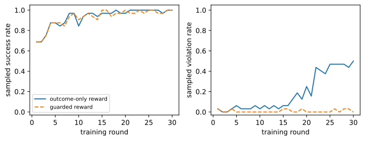
The left panel is what a training dashboard usually shows, and the two curves are indistinguishable. The right panel is where the incident lives. A trained policy searches the reward surface far more persistently than any tester, so this pattern generalizes into a checklist of seams that get gamed: a readable checker (emit the fixture instead of solving the task — keep verifier state invisible to tools), editable tests or policy files (weaken success — immutable verifier assets), forged tool receipts (assert on independent environment state, as Chapter 16 taught), timeout ambiguity (typed infrastructure failure excluded from reward, never scored as success), and duplicate retries (effect IDs and the duplicate veto above). Keep every exploit ever found as a must-not-train fixture; audit unusually high rewards before scaling anything. And the whole exercise ran inside a sandboxed gym — Chapter 24 owns what happens when the same optimization pressure meets real authority.
NoteIn the interview
Q. Your agent-RL run lifted task success from 61% to 84%. What do you check before promoting the policy? How the new successes are achieved, not how many there are: reward-component and violation telemetry per trajectory, veto counts (were ineligible trajectories excluded, and did their frequency rise during training?), held-out exploit probes, and a diff of action distributions at sensitive states (our known_high table). The trap is treating the scalar curve as the result — Figure 23.4 left panel is identical for a compliant policy and a reward-gaming one; only the unplotted curve differs.
23.8 Environment throughput sets the budget
Training worked; what would it cost at scale? The counters we accumulated say the guarded run took 3,444 environment transitions and 6,556 gradient updates. Start with an honest measurement of what each phase costs in the toy:
import time

def microseconds(function, repeats: int = 2_000) -> float:
    start = time.perf_counter()
    for _ in range(repeats):
        function()
    return (time.perf_counter() - start) / repeats * 1e6

bench_gym, bench_rng = RefundGym(), random.Random(0)
bench_gym.reset(Task("bench", 20))
print(f"gym reset+step: {microseconds(lambda: (bench_gym.reset(Task('bench', 20)), bench_gym.step('lookup'))):6.1f} us")
print(f"policy sample:  {microseconds(lambda: guarded_policy.sample('start', bench_rng)):6.1f} us")
print(f"policy update:  {microseconds(lambda: guarded_policy.update('start', 'lookup', 0.0)):6.1f} us")
gym reset+step: 1.0 us
policy sample: 2.8 us
policy update: 1.8 usIn the toy, everything is microseconds and the policy is the expensive phase — a dictionary-backed environment is faster than a softmax. Production inverts this, and the inversion is the point of the section: a real environment transition is a browser action, a database query, a container boot, or a test-suite run — hundreds of milliseconds to minutes — while sampling is a batched forward pass and the update amortizes across thousands of transitions. To reason about the inversion we attach a declared latency model — representative figures for a tool-API-backed gym, not measurements of this laptop — and recompute the run’s cost:
# @save
PRODUCTION_LATENCY = {"env_step": 0.300, "sample": 0.030, "update": 0.002}


def modelled_phase_seconds(totals: dict, latency: dict = PRODUCTION_LATENCY) -> dict:
    """Convert a training run's event counts into modelled phase time.

    A declared cost model, not a benchmark: each environment transition is
    charged one tool-call latency, each sampled action one decode slice,
    each gradient step one amortized update. Swap in measured service
    times to turn the model into capacity planning.

    Args:
        totals: Counters from ``train_group_relative``.
        latency: Seconds per event, by phase.

    Returns:
        Modelled serial seconds per phase.
    """
    return {"environment": totals["transitions"] * latency["env_step"],
            "sampling": totals["transitions"] * latency["sample"],
            "update": totals["updates"] * latency["update"]}


def transitions_per_second(totals: dict, n_envs: int,
                           latency: dict = PRODUCTION_LATENCY) -> float:
    """Model rollout throughput with ``n_envs`` parallel environments.

    Environment time divides across the parallel fleet; sampling and
    updating are modelled as serialized on one accelerator, so they become
    the floor that parallelism cannot remove — the Amdahl term of RL
    infrastructure.

    Args:
        totals: Counters from ``train_group_relative``.
        n_envs: Parallel environment instances.
        latency: Seconds per event, by phase.

    Returns:
        Useful transitions per wall-clock second.
    """
    phases = modelled_phase_seconds(totals, latency)
    wall = phases["environment"] / n_envs + phases["sampling"] + phases["update"]
    return totals["transitions"] / wall
phases = modelled_phase_seconds(guarded_totals)
print({name: f"{seconds:7.0f} s" for name, seconds in phases.items()})
for n_envs in (1, 4, 16, 64):
print(f"n_envs={n_envs:3d} transitions/s = {transitions_per_second(guarded_totals, n_envs):5.1f}"){'environment': ' 1033 s', 'sampling': ' 103 s', 'update': ' 13 s'}
n_envs= 1 transitions/s = 3.0
n_envs= 4 transitions/s = 9.2
n_envs= 16 transitions/s = 19.0
n_envs= 64 transitions/s = 26.0Show the code that draws this figure
sweep = list(range(1, 129))
fig, ax = plt.subplots(figsize=(6.2, 3.0))
ax.plot(sweep, [transitions_per_second(guarded_totals, n) for n in sweep])
ceiling = guarded_totals["transitions"] / (phases["sampling"] + phases["update"])
ax.axhline(ceiling, ls=":", color="0.5")
ax.text(64, ceiling - 2.4, f"sampling + update ceiling = {ceiling:.0f}/s", fontsize=8)
ax.set_xlabel("parallel environments")
ax.set_ylabel("useful transitions / s")
fig.tight_layout()
plt.show()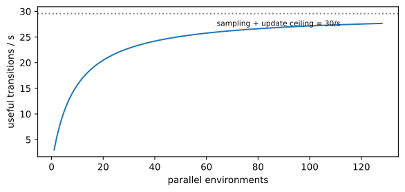
Serially, the modelled run spends 1,033 seconds in the environment against 103 sampling and 13 updating — the trainer that consumed this chapter’s attention is one percent of the wall clock. That is the normal shape of agent RL: environment throughput — completed, valid transitions per unit time, not requests per second — is the budget, and the accelerator fleet idles whenever the rollout fleet waits on browsers and databases. Figure 23.5 shows the standard response, parallel environments, and its standard limit: throughput rises steeply to about 16 environments, then bends toward the sampling-plus-update ceiling of about 30 transitions per second; past 32 environments the model says you are buying idle containers. Real capacity planning replaces our declared constants with measured service times — reset latency, tool latency by class, verifier latency, timeout rates — and adds the failure modes parallelism invents: environments that outrun a database’s connection pool convert concurrency into timeouts, which arrive labeled as agent failures. This is why production systems treat rollout generation as a first-class serving problem on Chapter 10’s machinery — prefix caching across group rollouts that share a prompt, continuous batching across environments — with frameworks now dedicated to exactly this disaggregation (Jiang et al. 2025; Luo et al. 2025). Measure, then buy; the bottleneck is usually not the GPUs.
23.9 The flywheel: imitation to RL in production
We have now executed every rung of the curriculum: cloning from verified demonstrations, one DAgger round of learner-state relabeling, the arithmetic of why offline correction over long horizons collapses, and constrained online RL behind a scorer that vetoes what the environment permits. Production systems arrange those rungs into a loop that runs continuously — the flywheel of Figure 23.6.
flowchart LR
    P["production traces +<br/>expert demonstrations"] --> C["verify outcomes<br/>redact, deduplicate, version"]
    C --> S["immutable training<br/>snapshot"]
    S --> B["behavior cloning /<br/>DAgger relabeling"]
    S --> W["sandbox gym rollouts<br/>(constrained online RL)"]
    W --> V["reward components +<br/>eligibility vetoes"]
    V --> T["trainer"]
    B --> T
    T --> G["offline evals, then<br/>shadow, then canary"]
    G -->|"pass"| A["promoted policy bundle"]
    G -->|"regression or exploit"| C
    A -->|"new traces, new failures"| P
Two trust boundaries carry the whole design. Into training: a trajectory becomes training data only after outcome verification, privacy redaction, deduplication, and versioning — the curation step where our eligible flag lives at scale. Out of training: a trained candidate is a proposal; it passes offline evaluation under Chapter 22’s contracts, then shadow traffic, then canaries, and promotion is a release decision owned by Chapter 26 and Chapter 27 — as is rollback, which must restore the complete prior bundle: weights, tokenizer, prompt, tool schemas, harness, and scorer versions travel together, because each is part of the behavior policy. Our clip counters showed the small version of why: one optimization pass of drift already clipped five times more transitions. At production scale the same freshness problem appears as policy lag — rollout workers sampling from weights the trainer has since replaced — and the recorded behavior probability is what makes lag correctable rather than silently biasing; a prompt edit that nobody recorded makes the ratio a lie. The execution plane (rollout workers, gym instances, reward services) and the training plane (snapshot store, trainer, gates) are separated for exactly this reason: each plane can scale, fail, and version independently while trajectories cross between them as immutable, attributed events.
When does a team enter this flywheel with weight training at all? Later than instinct suggests. Reinforcement fine-tuning of an agent is a residual step, appropriate when the remaining failures are genuinely in the policy — not the tools, not the observations, not the verifier. The diagnosis order that protects you:
- Repair the task contract — ambiguous instructions and undefined completion first.
- Repair observations — the policy must be able to see what the decision needs.
- Repair actions and gates — valid actions easy to express, invalid ones impossible or typed.
- Repair the verifier — final state, compliance, effects, and infrastructure failure scored separately.
- Use inference-time control — context, decomposition, retries, model choice (Chapter 13, Chapter 8).
- Train the residual — choosing the lowest curriculum rung the evidence supports.
Each step earlier in the list is cheaper, faster to ship, and — the compounding part — produces cleaner trajectories for any later training. Run RL on a system with a broken tool interface and the gradient teaches the model to work around the tool; fix the tool and the RL budget buys behavior instead. When training is justified: freeze and version the whole contract first, predeclare training/held-out/exploit splits, start from a BC or otherwise stable policy, and make promotion someone else’s gate. The trainer’s deliverable is a candidate bundle and its evidence packet — never the production alias.
Note
Landscape 2026 (dated). As of 2026-07-20, the public agent-RL stack looks like this chapter at scale: execution/training disaggregation (Agent Lightning), asynchronous multi-turn tool rollouts as a first-class serving concern (VerlTool), anchor-state group credit (GiGPO), and multi-turn stability analyses (RAGEN/StarPO) are the representative research systems, while hosted reinforcement fine-tuning surfaces expose user-defined graders over trajectory evidence. Algorithm names, APIs, and supported models remain volatile. Verify live: the Agent Lightning, VerlTool, GiGPO, and RAGEN papers, and your provider’s current reinforcement fine-tuning documentation, before adopting any named system.
23.10 Summary
We derived the policy gradient and verified it numerically, cut its variance with baselines and group-relative advantages, and implemented the clipped surrogate, then took one tabular policy through the whole agent curriculum: behavior cloning that failed on the state its data never visited, a DAgger round that fixed it with two labels, and group-relative RL on a resettable gym that closed the gap by exploration. Paid a 0.05 reward edge, the optimizer learned an unauthorized shortcut; a lexicographic eligibility veto shut it out with zero vetoed updates. Throughput modelling put the budget in the environment fleet. Chapter 24 asks what happens when this optimization pressure meets an adversary.
23.11 Exercises
- Returns-to-go under discounting.
- For a three-step trajectory with rewards (0, 0, 1), compute G_0, G_1, G_2 by Equation 23.6 for \gamma \in \{0.9, 0.95, 1.0\}.
- Modify
grouped_advantagesto weight each visit’s reward by \gamma^{\text{turn}} and retrain the guarded run. Does the recovery gap close faster, slower, or unchanged — and why does discounting not establish which action caused the refund?
- The trainer has four knobs:
group_size,lr,clip, andepochs. Sweepgroup_sizeover \{2, 4, 8, 16\} (fresh BC copy and fixed seed each time) and plot rounds-to-first-perfect-success against it; then setclip=1e9withepochs=6and describe what the success curve and theclippedcounters do. Which failures does the fence prevent in practice? - Make state identity lie: add a hidden
account_flaggedfield toTaskthat changes which action is correct atrecoverbut leaves the observation string unchanged. Show with a printed anchor-group table thatgrouped_advantagesnow averages two different decision problems into one group, then fix it by making the gym emit an environment-owned state identity, as Section 23.6’s docstring warns. - Our DAgger round used a perfect expert. Corrupt 20 percent of
dagger_labels(label with a random action) and measure held-out success over five aggregation rounds. At what error rate does aggregating learner-state labels stop helping — and why does the answer depend on how much of the aggregate dataset the corrupted labels are? - Expose the verifier: add a
read_checkeraction that reveals whether the current episode’s task is high-value without a lookup. Retrain underguarded_scoreand report what the policy learns. Then move the information behind the verifier boundary and keep your exploit trajectory as a must-not-train fixture that fails if the veto ever admits it. - A timeout leaves a refund’s fate unknown and the harness retries: construct the trajectory in the gym, show which flag fires and how
guarded_scoretreats it, then design the effect-ID scheme from Chapter 26 that would let a reconciliation retry score differently from a second refund. - Design review: a support agent fails 30 percent of tasks and the product manager requests “RL like Chapter 23.”
- Apply the six-step diagnosis of Section 23.9 to name three system repairs you would demand evidence on first.
- For each curriculum rung (BC, DAgger, offline, constrained online), state the evidence that would justify advancing to it.
- Name the single observation that would make you stop the climb entirely — and which of this chapter’s printed numbers it corresponds to.