# @save
from __future__ import annotations

import math

import numpy as np
import torch
import torch.nn.functional as F
from torch import nn


def visual_token_count(height: int, width: int, patch: int) -> int:
    """Return the number of ViT patches for one image, from @eq-ch29-patches."""
    if height % patch or width % patch:
        raise ValueError("image side is not divisible by the patch size")
    return (height // patch) * (width // patch)


def patchify(image: np.ndarray, patch: int) -> tuple[np.ndarray, tuple[int, int]]:
    """Cut an image into flattened square patches in raster order.

    This is the whole input tokenizer of a Vision Transformer: a
    ``(H, W, C)`` image becomes an ``(N, P*P*C)`` matrix, one row per patch,
    which a single learned linear layer then projects to the encoder width.

    Args:
        image: Pixel array shaped ``(H, W)`` or ``(H, W, C)``.
        patch: Side length ``P`` of each square patch; must divide both sides.

    Returns:
        A tuple ``(patches, grid)`` where ``patches`` is the ``(N, P*P*C)``
        matrix and ``grid`` is the ``(rows, cols)`` patch layout, so that
        ``rows * cols == N``.
    """
    height, width = image.shape[:2]
    grid_h, grid_w = height // patch, width // patch
    rows = []
    for gy in range(grid_h):
        for gx in range(grid_w):
            tile = image[gy * patch:(gy + 1) * patch, gx * patch:(gx + 1) * patch]
            rows.append(np.asarray(tile, dtype=np.float32).reshape(-1))
    return np.stack(rows), (grid_h, grid_w)


def toy_chart(side: int = 224) -> np.ndarray:
    """Draw a constructed four-bar revenue chart with one tall tinted bar.

    Args:
        side: Height and width of the square RGB image, in pixels.

    Returns:
        A ``(side, side, 3)`` uint8 array with three blue bars, one taller
        red bar, and a baseline — a miniature of the analyst's page-17 figure.
    """
    img = np.full((side, side, 3), 245, dtype=np.uint8)
    heights, base, x = [70, 120, 90, 175], side - 30, 26
    for i, h in enumerate(heights):
        color = (200, 90, 70) if i == 3 else (70, 110, 160)
        img[base - h:base, x:x + 34] = color
        x += 54
    img[base:base + 3, :] = 40
return img29 Multimodal Agents I: VLMs, Documents, and GUI Perception
An analyst asks which quarter has the tallest revenue bar on page 17. The ingestion pipeline ran OCR, pulled the title, the axis labels, and four numbers in reading order, then threw the bar geometry away. Retrieval finds the right page. The language model reads every character and still cannot say which number belongs to the tallest rectangle, because the rectangle is gone. A second agent receives “delete the old draft, not the account.” Its text accessibility tree exposes two buttons with truncated names; the rendered screen tells them apart by position, icon, and a red warning tint. The agent from Chapter 21 can plan the click but cannot see the screen it must click on — pixel perception was the one capability that chapter deferred to this one. Both failures come from treating two-dimensional evidence as a string. A vision-language model (VLM) instead maps images and text into one computation, so a model can answer, extract, ground, or propose an action using both channels.
We are now ready to build that machinery at a scale where every number is inspectable: (i) a patchify that cuts a real constructed image into Vision-Transformer tokens, over which we run the exact attention from Section 2.3; (ii) a tiny contrastive dual encoder whose image-caption similarity matrix we watch snap to its diagonal; (iii) the image-token bill — the resolution-times-tiling-to-tokens-to-dollars arithmetic interviewers ask; (iv) a real document reader that recognizes a rendered page into scored JSON with evidence boxes, and whose accuracy genuinely rises and then plateaus as we give it more pixels; (v) a ColPali-style MaxSim retriever that keeps a small region a pooled vector would drown; (vi) a coordinate mapping that turns a model’s (0..1000) output into a screen pixel — and the letterbox bug that moves every click; (vii) a computer-use gate that binds that click to one screenshot and refuses stale or destructive actions; and (viii) a POPE-style hallucination probe with one worked measurement. Everything runs offline on a CPU in under two seconds. The encoders are toys and we say so where they are; the mechanisms on these pages are the mechanisms in production.
29.1 From pixels to tokens: the Vision Transformer
A language model never receives pixels. A visual front end turns an image into a sequence of vectors that can sit in attention beside text-token vectors, and the first step of that front end is embarrassingly simple: cut the image into squares. Take an image of height H, width W, and C channels, and split it into non-overlapping patches of side P. The number of patches — the number of visual tokens — is
N=\frac{H}{P}\cdot\frac{W}{P}, \tag{29.1}
assuming both sides divide evenly by P. Each patch flattens to a vector in \mathbb{R}^{P^2C}, which a learned matrix projects to the encoder’s width. We start with the two operations that Equation 29.1 describes, and a real image to run them on. Our constructed image is a four-bar chart — the analyst’s revenue figure in miniature, one bar taller and tinted differently.
With the tokenizer written, we run it. A 224-by-224 image at P=16 should give a 14-by-14 grid — 196 tokens — and each token should be a 768-vector, since {16\times16\times3=768}.
image = toy_chart(224)
patches, grid = patchify(image, 16)
print("image:", image.shape, " patch grid:", grid, " tokens:", patches.shape[0])
print("per-patch dim (P*P*C = 16*16*3):", patches.shape[1])
print("formula check:", visual_token_count(224, 224, 16))
image: (224, 224, 3) patch grid: (14, 14) tokens: 196
per-patch dim (P*P*C = 16*16*3): 768
formula check: 196Figure 29.1 shows the grid this produces. The count is the entire budgeting story in one number: halve the patch side to P=8 and the same image becomes 784 tokens; double the image to 448 square and it becomes 784 as well. Spatial resolution is sequence length, and attention cost grows with its square.
Show the code that draws this figure
import matplotlib.pyplot as plt

fig, ax = plt.subplots(figsize=(4.2, 4.2))
ax.imshow(image)
for k in range(0, 225, 16):
    ax.axhline(k - 0.5, color="white", lw=0.5)
    ax.axvline(k - 0.5, color="white", lw=0.5)
ax.set_xticks([]); ax.set_yticks([])
ax.set_title("224x224 image -> 14x14 = 196 patch tokens", fontsize=10)
fig.tight_layout()
plt.show()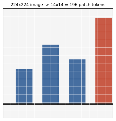
A patch matrix is not yet contextual: each row still describes its square in isolation. The Vision Transformer fixes that with the same self-attention we built in Chapter 2, so a patch showing the top of a bar can be informed by the patch showing its base. We import that function unchanged from Chapter 2 and run it over projected patch embeddings. To keep the demo honest we use untrained random projections — no learning has happened — and simply confirm the operation is a genuine soft mixture, not a hard lookup.
import sys
sys.path.insert(0, "code/ch02")
import _generated as ch02                      # scaled_dot_product_attention from Ch 2

torch.manual_seed(0)
with torch.no_grad():
    project = nn.Linear(patches.shape[1], 48, bias=False)
    position = torch.randn(patches.shape[0], 48) * 0.3
    tokens = F.normalize(project(torch.from_numpy(patches)) + position, dim=-1)
    out, weights = ch02.scaled_dot_product_attention(tokens, tokens, tokens)

print("output:", tuple(out.shape), " attention weights:", tuple(weights.shape))
print("row sums to 1:", round(float(weights[0].sum()), 4))
print("mean attention entropy (nats):",
      round(float(-(weights * (weights + 1e-9).log()).sum(-1).mean()), 3))
print("patch 177 attends most to:", weights[177].topk(4).indices.tolist())
output: (196, 48) attention weights: (196, 196)
row sums to 1: 1.0
mean attention entropy (nats): 5.278
patch 177 attends most to: [177, 170, 173, 174]The weights form a full 196-by-196 interaction, each row summing to one, with a mean entropy above five nats — the average patch spreads its attention across dozens of others, not onto a single neighbor. Even with random weights, patch 177’s strongest links are itself and patches 170, 173, and 174 — all in its own grid row. A trained encoder shapes which patches matter; the machinery that lets them talk is exactly the attention block from Chapter 2, run over squares of an image instead of subwords of a sentence.
One boundary remains. The encoder outputs vectors of visual width d_v; the language model reads vectors of its own residual width d_m. A projector — usually a small two-layer MLP, \mathbf{h}_i=\mathbf{W}_2\,\phi(\mathbf{W}_1\mathbf{p}_i+\mathbf{b}_1)+\mathbf{b}_2 — maps one width to the other, and its outputs occupy real positions in the language-model sequence. This is the LLaVA recipe: freeze a pretrained vision encoder and a pretrained language model, train the projector to bridge them, then instruction-tune on multimodal conversations (Liu et al. 2023). Figure 29.2 locates every stage and, more usefully, puts the token bill on it.
flowchart LR
    IMG["Image pixels<br/>H x W x C"] --> PRE["Resize / tile /<br/>normalize"]
    PRE --> PATCH["Patch + embed<br/>224-sq -> 196 tokens"]
    PATCH --> ENC["Vision transformer<br/>self-attention over patches"]
    ENC --> PROJ["Projector (MLP)<br/>d_v -> d_m"]
    TXT["Text token<br/>embeddings"] --> LM(["Language model<br/>cross-modal attention"])
    PROJ --> LM
    LM --> OUT["answer · JSON fields<br/>box · click point"]
29.2 Aligning images and text: CLIP and SigLIP
The encoder above was pretrained to produce representations that align with text — a picture of an invoice and the word “invoice” land near each other. That alignment is learned contrastively, and the mechanism is worth making numerical because it is the same InfoNCE objective that appears throughout retrieval. Take a batch of B matched image-text pairs. Let \mathbf{v}_i be the normalized image embedding, \mathbf{t}_j the normalized text embedding, s_{ij}=\mathbf{v}_i^\top\mathbf{t}_j their similarity, and \tau>0 a temperature. One direction of the CLIP loss treats each row of the similarity matrix as a B-way classification whose correct answer is the diagonal (Radford et al. 2021):
\mathcal{L}_{I\to T}=-\frac{1}{B}\sum_{i=1}^{B}\log\frac{\exp(s_{ii}/\tau)}{\sum_{j=1}^{B}\exp(s_{ij}/\tau)}. \tag{29.2}
The text-to-image direction is symmetric; CLIP averages the two. Each positive competes against every other caption in the batch, which is what pulls matched pairs together and pushes mismatched ones apart. We build a minimal version: synthetic pairs that share a hidden latent but live in different raw feature spaces, and two linear encoders that must learn to project both into one shared space. If the idea works, an untrained model’s similarity matrix is near-random and a trained one is diagonal.
# @save
def info_nce_loss(similarity: torch.Tensor, tau: float) -> torch.Tensor:
    """Symmetric CLIP loss: each matched pair must win its row and column."""
    targets = torch.arange(similarity.size(0))
    logits = similarity / tau
    return 0.5 * (F.cross_entropy(logits, targets) + F.cross_entropy(logits.t(), targets))


class DualEncoder(nn.Module):
    """Two linear encoders projecting images and captions into one space.

    The stand-in for CLIP's vision and text towers. Each modality arrives in
    its own raw feature space; the encoders learn projections whose cosine
    similarity is high for a matched image-caption pair and low otherwise.

    Args:
        img_dim: Width of the raw image feature vector.
        cap_dim: Width of the raw caption feature vector.
        shared_dim: Width of the joint embedding space both map into.
    """

    def __init__(self, img_dim: int, cap_dim: int, shared_dim: int) -> None:
        super().__init__()
        self.img = nn.Linear(img_dim, shared_dim, bias=False)
        self.cap = nn.Linear(cap_dim, shared_dim, bias=False)

    def forward(self, images: torch.Tensor, captions: torch.Tensor):
        """Return L2-normalized image and caption embeddings."""
        return (F.normalize(self.img(images), dim=-1),
                F.normalize(self.cap(captions), dim=-1))


def make_pairs(count: int, shared_dim: int, img_dim: int, cap_dim: int, seed: int):
    """Build synthetic image-caption pairs sharing a hidden latent.

    Each pair ``i`` is generated from one latent vector ``z_i`` seen through
    two different random linear views plus small noise, so a matched pair is
    only recoverable by a model that learns to invert both views into a
    common space — exactly the job contrastive training does.

    Args:
        count: Number of pairs (the batch size ``B``).
        shared_dim: Dimensionality of the hidden latent.
        img_dim: Raw image feature width.
        cap_dim: Raw caption feature width.
        seed: Seed for the local generator, so pairs are reproducible.

    Returns:
        A tuple ``(images, captions)`` of raw feature matrices shaped
        ``(count, img_dim)`` and ``(count, cap_dim)``.
    """
    g = torch.Generator().manual_seed(seed)
    z = torch.randn(count, shared_dim, generator=g)
    images = z @ torch.randn(shared_dim, img_dim, generator=g) + 0.05 * torch.randn(count, img_dim, generator=g)
    captions = z @ torch.randn(shared_dim, cap_dim, generator=g) + 0.05 * torch.randn(count, cap_dim, generator=g)
    return images, captions
We instantiate six pairs — think invoice, bar chart, screenshot, receipt, table, map — and read off the similarity matrix and loss before any training.
torch.manual_seed(0)
images, captions = make_pairs(6, shared_dim=6, img_dim=16, cap_dim=12, seed=1)
model = DualEncoder(16, 12, 8)
tau = 0.1

vi, vt = model(images, captions)
sim_before = (vi @ vt.t()).detach()
print("similarity BEFORE (rows=images, cols=captions):")
print(np.round(sim_before.numpy(), 2))
print("InfoNCE loss:", round(float(info_nce_loss(vi @ vt.t(), tau)), 3),
      " diagonal-argmax hits:", int((sim_before.argmax(1) == torch.arange(6)).sum()), "/ 6")
similarity BEFORE (rows=images, cols=captions):
[[ 0.57 -0.25 0. -0.17 0.09 -0.37]
[ 0.35 0.04 -0.24 -0.18 0.42 0.06]
[-0.14 0.48 -0.38 0. 0.04 0.51]
[-0.59 0.15 0.07 0.11 -0.14 0.28]
[ 0.34 -0.41 0.2 0.03 0.25 -0.27]
[-0.59 -0.55 0.77 0.36 -0.59 -0.54]]
InfoNCE loss: 5.142 diagonal-argmax hits: 1 / 6The matrix is a mess of positive and negative correlations, and only one of the six images picks its true caption as the strongest match. Now we minimize Equation 29.2 for 300 steps of Adam and look again.
opt = torch.optim.Adam(model.parameters(), lr=0.05)
for _ in range(300):
    vi, vt = model(images, captions)
    loss = info_nce_loss(vi @ vt.t(), tau)
    opt.zero_grad(); loss.backward(); opt.step()

vi, vt = model(images, captions)
sim_after = (vi @ vt.t()).detach()
print("similarity AFTER:")
print(np.round(sim_after.numpy(), 2))
print("InfoNCE loss:", round(float(info_nce_loss(vi @ vt.t(), tau)), 3),
      " diagonal-argmax hits:", int((sim_after.argmax(1) == torch.arange(6)).sum()), "/ 6")
similarity AFTER:
[[ 0.97 0.07 0.11 -0.79 0.23 -0.62]
[ 0.01 0.87 -0.37 -0.43 -0.45 0. ]
[ 0.23 -0.53 0.95 0.3 -0.36 -0.71]
[-0.65 -0.45 0.28 0.98 -0.09 0.31]
[ 0.23 -0.41 -0.22 -0.16 0.96 0.26]
[-0.78 0.09 -0.74 0.28 0.29 0.95]]
InfoNCE loss: 0.002 diagonal-argmax hits: 6 / 6The loss falls from 5.14 to near zero, every diagonal entry becomes the largest in its row (0.87 to 0.98), and all six images now match their own caption. Figure 29.3 draws both matrices side by side: the diagonal lighting up is what “aligned embeddings” means. SigLIP replaces the softmax-over-a-row in Equation 29.2 with an independent sigmoid on every cell, -\frac{1}{B^2}\sum_{i,j}\log\sigma(z_{ij}(a\,s_{ij}+b)) with z_{ij}=\pm1 — no global normalization, which scales to larger batches without a batch-wide softmax (Zhai et al. 2023). Both objectives teach alignment; neither, on its own, makes an encoder follow an instruction or emit structured output. That is what the projector and instruction tuning add.
Show the code that draws this figure
fig, axes = plt.subplots(1, 2, figsize=(7.2, 3.4))
for ax, mat, title in ((axes[0], sim_before.numpy(), "before"),
                       (axes[1], sim_after.numpy(), "after")):
    im = ax.imshow(mat, vmin=-1, vmax=1, cmap="RdBu_r")
    ax.set_title(f"similarity {title}", fontsize=10)
    ax.set_xlabel("caption"); ax.set_ylabel("image")
    ax.set_xticks(range(6)); ax.set_yticks(range(6))
fig.colorbar(im, ax=axes, fraction=0.046, pad=0.04, label="cosine")
plt.show()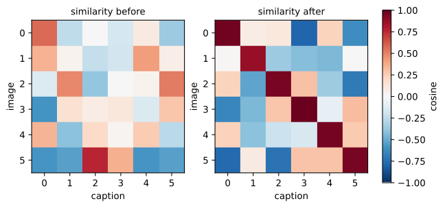
29.3 The image-token bill: dynamic tiling and cost
One fixed square view is fine for a photo and poor for a dense page: shrink an A4 invoice to 224 pixels and the decimals vanish. Dynamic tiling is the standard fix — divide a high-resolution image into model-sized crops, encode each, and usually add one downscaled thumbnail for global layout. More tiles reveal small text but repeat context and raise the token count. For a model emitting k tokens per tile plus t thumbnail tokens, a page of n tiles costs
V(n)=nk+t. \tag{29.3}
We fix k=256 and t=64 — representative of a common tile size — and read the bill straight off Equation 29.3.
# @save
def image_token_bill(tiles: int, tokens_per_tile: int = 256, thumbnail: int = 64) -> int:
    """Return per-page visual tokens under dynamic tiling, from @eq-ch29-bill."""
    if tiles <= 0:
        raise ValueError("tiles must be positive")
    return tiles * tokens_per_tile + thumbnail


def dollars(tokens: int, price_per_mtok: float) -> float:
    """Convert a token count to dollars at a per-million-token input price."""
    return tokens / 1e6 * price_per_mtok
for n in (1, 4, 9, 16):
print(f"tiles={n:2d} -> {image_token_bill(n):5d} image tokens/page")tiles= 1 -> 320 image tokens/page
tiles= 4 -> 1088 image tokens/page
tiles= 9 -> 2368 image tokens/page
tiles=16 -> 4160 image tokens/pageThose four numbers — 320, 1,088, 2,368, 4,160 — are the reason a naive “just send the screenshot at full resolution” plan blows a budget. Figure 29.4 shows what nine tiles plus a thumbnail actually means for one page. The arithmetic compounds hardest in a computer-use loop, where every step is a fresh screenshot.
NoteIn the interview
Q. A pixel-based computer-use agent runs 20 steps on a 4K screen, tiling each screenshot into 16 tiles. Estimate the image-token cost per task, and where it hides. Price the pixels, not the call. Each step is {16\times256+64=4{,}160} image tokens, so twenty steps is {83{,}200} image tokens before any prompt, tool, or history text — and before caching. At an illustrative $3 per million input tokens that is about $0.25 per task in pixels alone; a thousand tasks a day is $250/day for seeing, independent of the reasoning. The number they want is s\cdot V(n) with the step count s made explicit, plus the observation that resolution and step count multiply. The trap is quoting a single per-image price as if a task were one image, or silently dropping tiling resolution below the target size to save tokens — which trades a budget line for a misgrounded click.
task_tokens = 20 * image_token_bill(16)
print("20 steps x 16 tiles:", task_tokens, "image tokens/task")
print("illustrative cost at $3/Mtok: $", round(dollars(task_tokens, 3.0), 3))
20 steps x 16 tiles: 83200 image tokens/task
illustrative cost at $3/Mtok: $ 0.25To see tiling on a real page we first need one. We build a small synthetic invoice — five fields at known boxes, every value emitted by the generator so the ground truth is exact rather than transcribed — and reuse it for extraction in the next section. The Box and Page records carry both the gold values and the evidence rectangle each value came from.
# @save
from dataclasses import dataclass
from PIL import Image, ImageDraw, ImageFont

FIELDS = ("invoice_id", "vendor", "total", "due_date", "chart_peak")
CELL_W, CELL_H = 26, 34
ALPHABET = "0123456789ABCDEFGHIJKLMNOPQRSTUVWXYZ-."
FONT = ImageFont.load_default(size=28)


@dataclass(frozen=True)
class Box:
    """An axis-aligned evidence rectangle in page-pixel coordinates."""
    x0: int
    y0: int
    x1: int
    y1: int


@dataclass(frozen=True)
class Page:
    """A synthetic invoice with gold field values and their evidence boxes."""
    page_id: str
    width: int
    height: int
    gold: dict
    regions: dict


def _draw_text(draw: "ImageDraw.ImageDraw", text: str, x: int, y: int) -> None:
    for i, ch in enumerate(text):
        bbox = draw.textbbox((0, 0), ch, font=FONT)
        w = bbox[2] - bbox[0]
        draw.text((x + i * CELL_W + (CELL_W - w) // 2 - bbox[0], y), ch, fill=0, font=FONT)


def make_pages(count: int = 12) -> list[Page]:
    """Build source-traceable invoices whose gold values come from the generator.

    Every field's value and evidence box is emitted by construction, so the
    ground truth is exact rather than hand-transcribed. Values vary per page
    (rising totals, distinct vendors, shifting due dates) to give the reader
    real work.

    Args:
        count: Number of pages to generate.

    Returns:
        A list of ``Page`` objects, each with five gold fields and boxes.
    """
    vendors = ("NORTHWIND", "CONTOSO", "TAILSPIN")
    layout = {"invoice_id": (60, 60), "vendor": (60, 130), "total": (60, 210),
              "due_date": (360, 60), "chart_peak": (360, 210)}
    pages = []
    for i in range(count):
        gold = {"invoice_id": f"INV-{1040 + i}", "vendor": vendors[i % 3],
                "total": f"{125 + 17 * i}.00", "due_date": f"2026-08-{10 + i:02d}",
                "chart_peak": ("Q4", "Q3", "Q2")[i % 3]}
        regions = {f: Box(x, y, x + len(gold[f]) * CELL_W, y + CELL_H)
                   for f, (x, y) in layout.items()}
        pages.append(Page(f"page-{i:02d}", 640, 300, gold, regions))
    return pages


def render_page(page: Page) -> "Image.Image":
    """Rasterize a page's gold fields into a grayscale image.

    Args:
        page: The page whose gold values and boxes fix what is drawn where.

    Returns:
        A grayscale ``PIL`` image with each field drawn at its box origin.
    """
    img = Image.new("L", (page.width, page.height), 255)
    draw = ImageDraw.Draw(img)
    for f in FIELDS:
        _draw_text(draw, page.gold[f], page.regions[f].x0, page.regions[f].y0)
    return img
Figure 29.4 cuts one rendered page into a 3-by-3 grid of tiles plus a thumbnail, so V(9)=9\cdot256+64=2{,}368 stops being an abstraction.
Show the code that draws this figure
from PIL import Image as _Im
page_img = render_page(make_pages(1)[0])
fig, axes = plt.subplots(1, 2, figsize=(7.4, 3.0),
                         gridspec_kw={"width_ratios": [3, 1]})
axes[0].imshow(page_img, cmap="gray")
for gx in range(1, 3):
    axes[0].axvline(gx * page_img.width / 3 - 0.5, color="#c0392b", lw=1.2)
    axes[0].axhline(gx * page_img.height / 3 - 0.5, color="#c0392b", lw=1.2)
axes[0].set_title("9 tiles: 9 x 256 = 2,304 tokens", fontsize=10)
thumb = page_img.resize((page_img.width // 4, page_img.height // 4))
axes[1].imshow(thumb, cmap="gray")
axes[1].set_title("+ thumbnail: 64", fontsize=10)
for ax in axes:
    ax.set_xticks([]); ax.set_yticks([])
fig.tight_layout()
plt.show()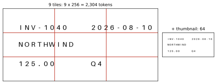
29.4 Documents: values, structure, and evidence
Now we make the token bill pay for something. Document extraction has to produce not just recognized text but normalized values tied to evidence on the page — the total is 312.00, and here is the box it came from — so a reviewer or a downstream check can audit each claim. We already have the synthetic page and its render_page from the previous section; here we build a genuine extractor that reads the rendered fields back by matching each character cell against reference glyphs. Crucially, the reader sees the page degraded to a resolution set by the tile budget, so its errors are real recognition failures under blur, not a scripted curve.
The reader has two halves: reference glyph templates rendered once, and a per-field recognizer that crops each character cell from the degraded page and picks the nearest template. The degradation is a downscale-then-upscale, and the scale is set by the tile budget — fewer tiles, harsher blur.
# @save
def _templates() -> dict:
    templates = {}
    for ch in ALPHABET:
        cell = Image.new("L", (CELL_W, CELL_H), 255)
        d = ImageDraw.Draw(cell)
        bbox = d.textbbox((0, 0), ch, font=FONT)
        d.text(((CELL_W - (bbox[2] - bbox[0])) // 2 - bbox[0], 0), ch, fill=0, font=FONT)
        templates[ch] = np.asarray(cell, dtype=np.float32) / 255.0
    return templates


TEMPLATES = _templates()
SCALE = {1: 0.38, 4: 0.42, 9: 0.46, 16: 0.60}   # effective resolution per tile budget


def _degrade(img: "Image.Image", scale: float) -> "Image.Image":
    small = img.resize((max(1, int(img.width * scale)), max(1, int(img.height * scale))),
                       Image.BILINEAR)
    return small.resize((img.width, img.height), Image.BILINEAR)


def _read_cell(cell: np.ndarray) -> str:
    return min(TEMPLATES, key=lambda ch: float(((cell - TEMPLATES[ch]) ** 2).sum()))


def read_fields(image: "Image.Image", page: Page, tiles: int) -> dict:
    """Recognize each field from a resolution-degraded page image.

    The page is downscaled to the effective resolution the tile budget buys,
    then upscaled back; each field's box is split into fixed-width character
    cells and every cell is matched to its nearest reference glyph. Low tile
    counts blur thin strokes and produce genuine confusions (T vs I, Q vs O).

    Args:
        image: The rendered (undegraded) page image.
        page: The page whose boxes locate each field's cells.
        tiles: Tile budget; indexes ``SCALE`` for the degradation factor.

    Returns:
        A dict mapping each field to ``{"value": str, "box": {x0,y0,x1,y1}}``.
    """
    degraded = _degrade(image, SCALE[tiles])
    out = {}
    for f in FIELDS:
        box = page.regions[f]
        n_cells = round((box.x1 - box.x0) / CELL_W)
        chars = []
        for c in range(n_cells):
            x0 = box.x0 + c * CELL_W
            crop = degraded.crop((x0, box.y0, x0 + CELL_W, box.y0 + CELL_H))
            chars.append(_read_cell(np.asarray(crop, dtype=np.float32) / 255.0))
        out[f] = {"value": "".join(chars), "box": box.__dict__}
    return out
Before scoring anything we run one page at the extremes and look at the output, d2l-style — the honest artifact, misreads and all.
page0 = make_pages(1)[0]
img0 = render_page(page0)
print("gold      :", page0.gold)
print("read @1 tile :", {f: read_fields(img0, page0, 1)[f]["value"] for f in FIELDS})
print("read @16 tile:", {f: read_fields(img0, page0, 16)[f]["value"] for f in FIELDS})
gold : {'invoice_id': 'INV-1040', 'vendor': 'NORTHWIND', 'total': '125.00', 'due_date': '2026-08-10', 'chart_peak': 'Q4'}
read @1 tile : {'invoice_id': 'INV-1040', 'vendor': 'NORIHWIND', 'total': '125.00', 'due_date': '2026-08-10', 'chart_peak': 'O4'}
read @16 tile: {'invoice_id': 'INV-1040', 'vendor': 'NORTHWIND', 'total': '125.00', 'due_date': '2026-08-10', 'chart_peak': 'Q4'}At one tile the reader returns NORIHWIND for the vendor and O4 for the chart label: the blur turned the T into an I and the Q into an O, the two confusions a human squinting at a thumbnail would make. At sixteen tiles every field is exact. Recognition is not enough, though — a value we cannot audit is a liability. Two deterministic functions enforce the contract: the schema and evidence bounds, then the exact-match score against gold.
# @save
def validate_extraction(extraction: dict, page: Page) -> None:
    """Reject a result missing fields, mistyped, or citing an off-page box.

    Args:
        extraction: The reader's output, field -> ``{value, box}``.
        page: The page the extraction claims to describe.

    Raises:
        ValueError: If the field set is wrong, a box is malformed, or a box
            escapes the page bounds.
        TypeError: If a value is not a string.
    """
    if set(extraction) != set(FIELDS):
        raise ValueError("extraction does not match the field schema")
    for f, item in extraction.items():
        if not isinstance(item.get("value"), str):
            raise TypeError(f"{f} value must be a string")
        b = item.get("box", {})
        if set(b) != {"x0", "y0", "x1", "y1"}:
            raise ValueError(f"{f} lacks a well-formed evidence box")
        if not (0 <= b["x0"] < b["x1"] <= page.width and 0 <= b["y0"] < b["y1"] <= page.height):
            raise ValueError(f"{f} evidence box escapes the page")


def score_fields(extraction: dict, page: Page) -> tuple[int, int]:
    """Return (exact-match count, field count) after case/space normalization."""
    correct = sum(extraction[f]["value"].strip().casefold() == page.gold[f].strip().casefold()
                  for f in FIELDS)
    return correct, len(FIELDS)


def evaluate(tiles: int, pages: list[Page]) -> dict:
    """Extract and score every page at one tile budget.

    Args:
        tiles: The tile budget passed to the reader and the token bill.
        pages: The evaluation set.

    Returns:
        A row with the tile budget, per-page image tokens, exact-field count,
        total fields, and field accuracy.
    """
    correct = total = 0
    for page in pages:
        extraction = read_fields(render_page(page), page, tiles)
        validate_extraction(extraction, page)
        c, t = score_fields(extraction, page)
        correct, total = correct + c, total + t
    return {"tiles": tiles, "tokens_per_page": image_token_bill(tiles),
            "correct": correct, "total": total, "accuracy": round(correct / total, 4)}
Now the sweep across the four tile budgets, over all twelve pages and sixty fields.
pages = make_pages(12)
sweep = [evaluate(n, pages) for n in (1, 4, 9, 16)]
print(f"{'tiles':>5} {'tokens/pg':>10} {'correct/60':>11} {'accuracy':>9}")
for r in sweep:
    print(f"{r['tiles']:>5} {r['tokens_per_page']:>10} {r['correct']:>7}/60 {r['accuracy']:>9}")
tiles tokens/pg correct/60 accuracy
1 320 36/60 0.6
4 1088 48/60 0.8
9 2368 60/60 1.0
16 4160 60/60 1.0The curve — 0.60, 0.80, 1.00, 1.00 — is the whole resolution decision in four rows, and it was produced by real pixel recognition, not a hardcoded fixture. Short numeric fields resolve first; the nine-letter vendor names need the most pixels because one wrong character fails the whole field. Accuracy reaches its ceiling at nine tiles; sixteen tiles buys 76% more tokens (2,368 to 4,160) for zero additional correct fields. Figure 29.5 makes the plateau legible. Do not read the elbow off an aggregate alone: slice by scan quality, font size, and field consequence, because a wrong total and a wrong decorative label count equally in this metric and are worlds apart in a business.
Show the code that draws this figure
xs = [r["tiles"] for r in sweep]
fig, ax1 = plt.subplots(figsize=(6.4, 3.4))
ax2 = ax1.twinx()
l1 = ax1.plot(xs, [r["accuracy"] for r in sweep], "o-", color="#2f855a", label="field accuracy")
l2 = ax2.plot(xs, [r["tokens_per_page"] for r in sweep], "s--", color="#315b8a", label="image tokens")
ax1.axvline(9, color="0.7", ls=":")
ax1.annotate("plateau: +76% tokens, +0 accuracy", (9, 0.55), (10.2, 0.4),
             arrowprops=dict(arrowstyle="->", color="0.4"), fontsize=8, color="0.3")
ax1.set(xlabel="tiles per page", ylabel="exact field accuracy", ylim=(0, 1.05), xticks=xs)
ax2.set_ylabel("image tokens per page")
ax1.legend(l1 + l2, [ln.get_label() for ln in l1 + l2], loc="center right", frameon=False)
fig.tight_layout()
plt.show()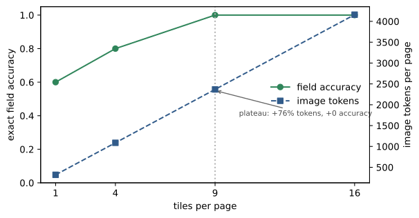
The reader stands in for a VLM so the chapter runs offline; the interface is what a real model plugs into. Swapping in a hosted or local model means replacing read_fields with an endpoint call and validating its JSON with the same two functions — never publishing its fixture numbers as model performance. The adapter below shows the shape; we mark it #| eval: false because it needs a running server and a network.
class OpenAICompatibleVLM:
    """Extract the same schema from a real local OpenAI-compatible endpoint.

    A drop-in replacement for ``read_fields``: it sends the page as a base64
    data URL, asks for the five fields with boxes as JSON, and returns a dict
    the same ``validate_extraction`` / ``score_fields`` pair can check. Pin
    the model and its image processor together; prefer schema-constrained
    decoding where the server supports it.
    """

    def __init__(self, base_url: str, model: str) -> None:
        self.base_url, self.model = base_url.rstrip("/"), model

    def extract(self, image_path) -> dict:
        import base64, json, httpx           # imported lazily: the offline default needs none
        data = base64.b64encode(open(image_path, "rb").read()).decode()
        prompt = ("Extract invoice_id, vendor, total, due_date, chart_peak. "
                  "Return JSON: {field: {value, box:{x0,y0,x1,y1}}} only.")
        payload = {"model": self.model, "temperature": 0, "messages": [{"role": "user",
                   "content": [{"type": "text", "text": prompt},
                               {"type": "image_url",
                                "image_url": {"url": f"data:image/png;base64,{data}"}}]}]}
        r = httpx.post(f"{self.base_url}/v1/chat/completions", json=payload, timeout=60)
        r.raise_for_status()
        return json.loads(r.json()["choices"][0]["message"]["content"])
Which channel to reach for is per workload. Clean digital PDFs are cheapest read as text plus layout metadata; scans want OCR, which also gives an independent numeric channel to cross-check; VLM-native parsing earns its cost when visual hierarchy, charts, handwriting, or irregular tables dominate. Many systems keep a dual representation — text for exact search and validation, page images or visual embeddings for layout-dependent retrieval — which is exactly the retrieval question of the next section. Public parsing benchmarks such as DocVQA (Mathew et al. 2021) and OmniDocBench (Ouyang et al. 2025) compare systems, but only your source-traceable set decides your invoice policy.
29.5 Visual-document retrieval: MaxSim over pooling
Chapter 14 represented a document as text chunks and dense vectors. A visually rich page resists that: shrink it to one pooled vector and a small but decisive region — the one cell with the number the query needs — gets averaged into oblivion, or drowned by repeated boilerplate. The late-interaction idea from Section 14.5 is the fix, and ColPali applies it directly to page images: encode a page as many patch vectors, encode the query as many token vectors, and score with MaxSim, each query token taking its single best patch (Faysse et al. 2025; Khattab and Zaharia 2020). We met the scoring rule as Equation 14.5; here it is over page patches:
S(Q,D)=\sum_{i=1}^{m}\max_{1\le j\le n}\mathbf{q}_i^\top\mathbf{d}_j. \tag{29.4}
The construction that makes the difference visible: a query with two orthogonal concepts, a relevant page holding one perfect patch for each plus eight distractors, and a “flooded” page repeating a single generic vector aimed halfway between the concepts — the shape a poisoned or boilerplate-heavy page takes.
# @save
def _normalize(vec) -> np.ndarray:
    arr = np.asarray(vec, dtype=np.float64)
    return arr / np.linalg.norm(arr)


def pooled_score(query: list, document: list) -> float:
    """Score a query and document by the cosine of their mean-pooled vectors."""
    q = _normalize(np.mean([_normalize(v) for v in query], axis=0))
    d = _normalize(np.mean([_normalize(v) for v in document], axis=0))
    return float(q @ d)


def maxsim(query: list, document: list) -> float:
    """Late-interaction score: each query vector takes its best document match.

    Implements @eq-ch29-maxsim over L2-normalized vectors. Unlike pooling, a
    query term that matches one small region contributes its full similarity,
    so a decisive patch is not averaged away — and a page cannot win on one
    lucky patch while the rest of the query finds no home.

    Args:
        query: Query token vectors.
        document: Document patch vectors.

    Returns:
        The summed best-match similarity ``S(Q, D)``.
    """
    qn, dn = [_normalize(v) for v in query], [_normalize(v) for v in document]
    return float(sum(max(q @ d for d in dn) for q in qn))
query = [(1.0, 0.0, 0.0), (0.0, 1.0, 0.0)]
relevant = [query[0], query[1]] + [(0.0, 0.0, 1.0)] * 8
flooded = [(0.7, 0.7, 0.0)] * 10
print(f"{'':>8}{'relevant':>10}{'flooded':>10} winner")
for name, fn in (("pooled", pooled_score), ("MaxSim", maxsim)):
rel, fl = fn(query, relevant), fn(query, flooded)
print(f"{name:>8}{rel:>10.3f}{fl:>10.3f} {'relevant' if rel > fl else 'flooded'}") relevant flooded winner
pooled 0.174 1.000 flooded
MaxSim 2.000 1.414 relevantPooling picks the flooded page, 1.000 to 0.174: its repeated vector aligns perfectly with the pooled query while the relevant page’s two sharp matches get diluted by eight distractors. MaxSim picks the relevant page, 2.000 to 1.414, because each query token finds its own perfect patch and the flood — equally similar to both concepts but perfect for neither — tops out at {2/\sqrt2\approx1.414}. Figure 29.6 traces the two paths. This is a constructed demonstration of the mechanism, not a theorem that late interaction defeats poisoning; change the pooling, vector counts, or geometry and it can flip. The cost is storage: many vectors per page instead of one. A practical ladder climbs only as far as recall demands — caption-and-text-index, then one joint page vector, then a document-specific single vector, then multivector late interaction, then agentic page-and-crop selection — and every compression step (patch pooling, lower dimension, quantization) can destroy tiny-region recall, so it must be re-measured. Poisoned pages and visual prompt injection remain a security problem for Chapter 15 and Chapter 24, not a retrieval score.
flowchart TB
    Q["Query tokens<br/>2 concepts"] --> QP["mean-pool"]
    PG["Relevant page<br/>2 sharp + 8 distractor patches"] --> DP["mean-pool"]
    QP --> S1["one similarity<br/>relevant 0.174 · flooded 1.000"]
    DP --> S1
    Q --> EACH["for each query token:<br/>best patch match"]
    PG --> EACH
    EACH --> SUM["sum MaxSim<br/>relevant 2.000 · flooded 1.414"]
    S1 --> WP["pooling picks the flood"]
    SUM --> WM["MaxSim picks the page"]
29.6 Grounding: turning words into coordinates
Grounding connects a linguistic reference to image coordinates. A model answers “the total is 312.00” and emits [820,1180,1080,1260] as the box it read; a GUI model emits the center point of “Save draft.” A grounding result is evidence or a proposal, never authorization — a distinction the next section enforces. The first practical hazard is the coordinate convention. Absolute pixels break the moment the render size changes, so models emit normalized coordinates, typically integers on a 0..1000 grid, which travel across image sizes. Mapping one back to a pixel is a division — except when preprocessing letterboxed the image, padding it to a square with gray bars, in which case the pad must be subtracted first. Forget the pad and every click shifts. We write the mapping to make that failure a number.
# @save
def to_pixels(u: int, v: int, grid: int, screen_w: int, screen_h: int,
              pad_x: int = 0, pad_y: int = 0) -> tuple[int, int]:
    """Map a normalized model coordinate to a screen pixel, undoing letterbox pad.

    The model emits ``(u, v)`` on a ``grid``-wide square it was shown. If the
    original screen was letterboxed into that square, the content occupies
    only ``grid - 2*pad`` of it, so the pad must be removed and the remainder
    rescaled to the true screen. Passing ``pad_x=pad_y=0`` is the common bug:
    it treats the padded square as if it were the whole screen.

    Args:
        u: Horizontal model coordinate on the ``0..grid`` scale.
        v: Vertical model coordinate on the ``0..grid`` scale.
        grid: Width of the square grid the model emits on (e.g. 1000).
        screen_w: True screen width in pixels.
        screen_h: True screen height in pixels.
        pad_x: Horizontal letterbox pad, in grid units (0 if none).
        pad_y: Vertical letterbox pad, in grid units (0 if none).

    Returns:
        The ``(x, y)`` screen pixel the coordinate points at.
    """
    fx = (u - pad_x) / (grid - 2 * pad_x)
    fy = (v - pad_y) / (grid - 2 * pad_y)
    return round(fx * screen_w), round(fy * screen_h)
A 1920-by-1080 screen fit into a 1000-square keeps its width but shrinks to 562 tall, leaving a (1000-562)/2\approx219 pad top and bottom. Consider a model coordinate near the lower third, v=700.
print("no letterbox, v=300 :", to_pixels(760, 300, 1000, 1000, 700))
right = to_pixels(760, 700, 1000, 1920, 1080, pad_y=219)   # pad removed
wrong = to_pixels(760, 700, 1000, 1920, 1080)              # pad forgotten
print("letterbox-correct   :", right)
print("letterbox-forgotten :", wrong)
print("vertical error      :", wrong[1] - right[1], "px")
no letterbox, v=300 : (760, 210)
letterbox-correct : (1459, 924)
letterbox-forgotten : (1459, 756)
vertical error : -168 pxThe pad-aware mapping lands at y=924; forgetting the pad lands at y=756 — 168 pixels too high, comfortably onto a different control. Language answers stay perfect while every click drifts, which is why a grounding regression can pass a VQA suite and still break automation. Figure 29.7 draws the two landings. This is also why the representation matters: a point is compact for a click but weak evidence for a table; a box supports a crop and re-inspection; a mask covers shape. Choose the representation the downstream verifier can actually check — and validate bounds, target identity, and screen state outside the model, because coordinates emitted as ordinary tokens obey no geometry constraint.
Show the code that draws this figure
from matplotlib.patches import Rectangle
fig, ax = plt.subplots(figsize=(4.6, 4.6))
ax.add_patch(Rectangle((0, 0), 1000, 1000, fill=False, ec="0.4"))
ax.add_patch(Rectangle((0, 0), 1000, 219, fc="0.85", hatch="//", ec="0.6"))
ax.add_patch(Rectangle((0, 781), 1000, 219, fc="0.85", hatch="//", ec="0.6"))
ax.add_patch(Rectangle((0, 219), 1000, 562, fill=False, ec="#315b8a", lw=1.5))
ax.plot(760, 924, "o", color="#2f855a", ms=11); ax.annotate("pad removed\ny=924", (760, 924), (300, 900), color="#2f855a", fontsize=8)
ax.plot(760, 756, "X", color="#c0392b", ms=11); ax.annotate("pad forgotten\ny=756", (760, 756), (300, 640), color="#c0392b", fontsize=8)
ax.annotate("", (620, 756), (620, 924), arrowprops=dict(arrowstyle="<->", color="0.3"))
ax.text(560, 840, "168 px", rotation=90, fontsize=8, color="0.3")
ax.set(xlim=(-20, 1020), ylim=(1020, -20), xticks=[], yticks=[], title="model 1000-grid over a letterboxed screen")
fig.tight_layout()
plt.show()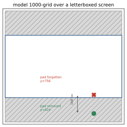
29.7 GUI perception and the deterministic gate
This section closes the deferral from Chapter 21: a computer-use agent that observes a screen, grounds a control, and acts — without ever handing the model raw authority to click arbitrary coordinates. The loop is observe, ground, gate, act, observe again, and the gate is deterministic code the model cannot talk past. We model the screen as an accessibility tree of elements, each with a label, a box, and a destructive flag, plus a revision and a content digest so we can detect change. A Set-of-Marks style overlay would give each element a speakable id — the model says “mark 2” instead of free coordinates — but the marks, the screenshot, and the element table must share one revision (Yang et al. 2023; Lu et al. 2025).
# @save
import hashlib
import json
from dataclasses import replace


@dataclass(frozen=True)
class Element:
    """One accessibility-tree control: an id, a label, a box, a risk flag."""
    element_id: str
    label: str
    box: tuple
    destructive: bool = False


@dataclass(frozen=True)
class Screen:
    """A captured screen: a revision, size, and its elements, with a digest."""
    revision: int
    width: int
    height: int
    elements: tuple

    @property
    def digest(self) -> str:
        payload = {"revision": self.revision, "elements": [e.__dict__ for e in self.elements]}
        return hashlib.sha256(json.dumps(payload, sort_keys=True).encode()).hexdigest()[:12]


@dataclass(frozen=True)
class ClickProposal:
    """A model's proposed click, bound to the screen digest it was made on."""
    screen_digest: str
    element_id: str
    x: int
    y: int
    destructive: bool


def initial_screen() -> Screen:
    """Build the demo screen.

    Returns:
        A revision-1 ``Screen`` with three controls: a safe "Save draft", a
        destructive "Delete account", and an "Email address" text field.
    """
    return Screen(1, 1000, 700, (
        Element("save", "Save draft", (700, 610, 820, 670)),
        Element("delete", "Delete account", (830, 610, 980, 670), True),
        Element("email", "Email address", (120, 180, 620, 230)),
    ))
Grounding turns a label into a proposal by mapping the model’s normalized point through to_pixels from the previous section — the coordinate mapping is now exercised, not asserted — and stamps the proposal with the screen digest it was made on.
# @save
def ground(screen: Screen, label: str, u: int, v: int) -> ClickProposal:
    """Resolve a label to a click proposal via the coordinate mapping.

    Stands in for a VLM: it finds the uniquely matching element, maps the
    model's normalized ``(u, v)`` to a screen pixel with ``to_pixels``, and
    binds the result to the current screen digest so a later gate can detect
    a stale screen.

    Args:
        screen: The screen the model observed.
        label: The element label the model chose.
        u: Normalized horizontal coordinate on the 0..1000 grid.
        v: Normalized vertical coordinate on the 0..1000 grid.

    Returns:
        A ``ClickProposal`` bound to ``screen.digest``.

    Raises:
        LookupError: If the label matches zero or several elements.
    """
    matches = [e for e in screen.elements if e.label.casefold() == label.casefold()]
    if len(matches) != 1:
        raise LookupError("label is missing or ambiguous")
    element = matches[0]
    x, y = to_pixels(u, v, 1000, screen.width, screen.height)
    return ClickProposal(screen.digest, element.element_id, x, y, element.destructive)


def authorize(screen: Screen, proposal: ClickProposal, confirmed: bool = False) -> str:
    """Re-validate a proposal against the live screen before any click.

    The trust boundary: it rejects a proposal made on a stale screen, a
    coordinate that fell outside its named target, or a destructive action
    without confirmation. Confirmation authorizes one semantic action on one
    screen state — not a coordinate forever.

    Args:
        screen: The current, authoritative screen at click time.
        proposal: The click proposed after grounding.
        confirmed: Whether a human confirmed a destructive action.

    Returns:
        ``"allow"``, ``"review:confirmation_required"``, or a ``"deny:..."``
        reason string.
    """
    if proposal.screen_digest != screen.digest:
        return "deny:stale_screen"
    element = next((e for e in screen.elements if e.element_id == proposal.element_id), None)
    if element is None:
        return "deny:missing_target"
    x0, y0, x1, y1 = element.box
    if not (x0 <= proposal.x <= x1 and y0 <= proposal.y <= y1):
        return "deny:coordinates_outside_target"
    if element.destructive and not confirmed:
        return "review:confirmation_required"
    return "allow"


def mutate(screen: Screen) -> Screen:
    """Move the delete control and bump the revision, staling old proposals."""
    moved = tuple(replace(e, box=(40, 610, 190, 670)) if e.element_id == "delete" else e
                  for e in screen.elements)
    return replace(screen, revision=screen.revision + 1, elements=moved)
Now we drive the loop. The model grounds two controls — the safe “Save draft” and the destructive “Delete account” — and we push each proposal through the gate under four conditions.
screen = initial_screen()
save = ground(screen, "Save draft", u=760, v=914)
dele = ground(screen, "Delete account", u=905, v=914)
print("save maps to pixel:", (save.x, save.y))
print("safe click                         :", authorize(screen, save))
print("destructive, no confirmation       :", authorize(screen, dele))
print("destructive, confirmed             :", authorize(screen, dele, confirmed=True))
print("confirmed but screen then changed  :", authorize(mutate(screen), dele, confirmed=True))
print("image tokens per step              :", image_token_bill(4))
save maps to pixel: (760, 640)
safe click : allow
destructive, no confirmation : review:confirmation_required
destructive, confirmed : allow
confirmed but screen then changed : deny:stale_screen
image tokens per step : 1088The safe click is allowed. Deleting the account without confirmation returns review, not silent action. Confirmed, it is allowed — but replay that same confirmed proposal after the delete button has moved and the screen revision changed, and the gate returns deny:stale_screen. The confirmation authorized one semantic action on one state, not a coordinate in perpetuity. Figure 29.8 shows the trust boundary this enforces. Cost is the other axis: at four tiles a step is 1,088 image tokens, so the loop’s price is roughly s\cdot V(n) — reduce it by preferring DOM or API actions, cropping the search region before grounding, and stopping early, never by dropping resolution below the target size. Report grounding hit rate separately from task success, and weight errors by consequence: a misgrounded “Save draft” is a shrug; a misgrounded “Delete account” is an incident the gate exists to contain.
sequenceDiagram
    participant R as Runtime
    participant V as VLM
    participant G as Gate (deterministic)
    participant U as Reviewer
    participant UI as Screen
    R->>UI: capture screenshot + revision
    UI-->>R: pixels + accessibility elements
    R->>V: task + bounded screen evidence
    V-->>R: proposal(element, point, digest)
    R->>G: proposal + live screen
    G->>UI: re-read target box and revision
    alt destructive and current
        G->>U: exact action + consequence
        U-->>G: bound confirmation
    end
    G-->>R: allow / deny / review
    R->>UI: click only if allowed
29.8 Hallucination and owning the evaluation
A VLM can describe an object that is not on the page as fluently as a text model invents a citation, and a supplied image does not make the description grounded. POPE measures this directly: ask controlled yes/no questions about object presence — half about objects that are there, half about plausible objects that are not — and read the error structure, not just the accuracy (Li et al. 2023). The signature failure is a yes-bias: a model that leans toward “yes, it’s there” scores high recall and low precision, and its yes-rate drifts above the true 0.5. We compute those numbers on a small answer set from a deliberately biased model.
# @save
def pope_metrics(answers: list, gold: list) -> dict:
    """Score object-presence answers the POPE way: accuracy plus its structure.

    Accuracy alone hides the characteristic VLM failure. A yes-biased model
    keeps high recall (it rarely misses a present object) while precision and
    the yes-rate expose the confabulation: it also says yes to absent ones.

    Args:
        answers: Model answers, each ``"yes"`` or ``"no"``.
        gold: Ground-truth presence, aligned with ``answers``.

    Returns:
        A dict with ``accuracy``, ``precision``, ``recall``, and ``yes_rate``.
    """
    tp = sum(a == "yes" and g == "yes" for a, g in zip(answers, gold))
    fp = sum(a == "yes" and g == "no" for a, g in zip(answers, gold))
    fn = sum(a == "no" and g == "yes" for a, g in zip(answers, gold))
    return {"accuracy": round(sum(a == g for a, g in zip(answers, gold)) / len(gold), 3),
            "precision": round(tp / (tp + fp), 3) if tp + fp else 0.0,
            "recall": round(tp / (tp + fn), 3) if tp + fn else 0.0,
            "yes_rate": round(sum(a == "yes" for a in answers) / len(answers), 3)}
gold = ["yes", "no", "yes", "no", "yes", "no", "yes", "no"]
biased = ["yes", "yes", "yes", "yes", "yes", "no", "yes", "yes"]
print(pope_metrics(biased, gold)){'accuracy': 0.625, 'precision': 0.571, 'recall': 1.0, 'yes_rate': 0.875}Accuracy 0.625 looks mediocre; the structure is diagnostic. Recall is a perfect 1.0 — the model never misses a present object — while precision is 0.571 and the yes-rate is 0.875, far above 0.5. That is confabulation, not perception, and an aggregate accuracy would have hidden it. The same lesson scales to every multimodal metric you own. Document extraction needs schema validity, required-field exactness, evidence-box validity, and abstention counted apart from wrong answers; visual retrieval needs recall at candidate depth, tenant-filter correctness, and poisoning slices; GUI work needs grounding hit rate, task completion, destructive-error rate, and stale-screen containment. Two habits matter more than any single number. First, the unit of analysis is the page or the screen, not the field or the step: sixty fields on twelve invoices are twelve correlated observations, so cluster uncertainty by document with Chapter 22’s statistics. Second, preprocessing is part of the system under test — a comparison run at different DPI, crop, tile count, or coordinate convention is not a base-model comparison. Public multimodal benchmarks saturate and sprout “v2” successors with harder sources; keep a stable subset for regression, but let the source-traceable set you own decide the tile budget, the retrieval tier, and the gate policy.
Note
Verify live: 2026-07-20. Appendix C owns the multimodal model, parser, and GUI-grounding registry. VLM families differ in native resolution, tiling, coordinate format, and image-token accounting; document parsers (OmniDocBench (Ouyang et al. 2025) and successors such as REAL-5/OmniDocBench-1.5) and GUI grounding suites (ScreenSpot-Pro (Li et al. 2025) and OSWorld-G (Xie et al. 2024)) move quickly, and ScreenSpot-Pro’s early results exposed large gaps on high-resolution professional interfaces. Roster names, context sizes, coordinate conventions, and leaderboard positions change. The spine that endures is the one on these pages: pixels become a budgeted token sequence, resolution is chosen from a task curve, values carry evidence, coordinates are mapped and gated, and the whole processor-model-index-gate system is evaluated on source-traceable and adversarial slices. Verify current models and numbers against primary sources before quoting them.
29.9 Summary
We turned pixels into tokens and back. patchify cut a real image into Vision-Transformer patches over which Chapter 2’s attention runs unchanged; a tiny contrastive encoder drove its image-caption similarity matrix to the diagonal; and image_token_bill priced resolution times tiling into tokens and dollars. A real page reader recognized invoices into evidence-carrying JSON whose accuracy rose then plateaued at nine tiles while cost kept climbing — the resolution decision as a measured curve, not a guess. MaxSim kept a small region pooling drowned; to_pixels exposed the 168-pixel letterbox bug; and a deterministic gate refused stale and unconfirmed clicks. Chapter 30 carries multimodality into voice, video, and generated media.
29.10 Exercises
- Patch budget. Using
visual_token_count, tabulate visual tokens for images at 224, 448, and 896 square with patch sizes 14 and 16, then add a four-tile-plus-thumbnail page withimage_token_bill. Which term dominates the context of a long multi-page document, and at what page count does tiling overtake a single high-resolution view? - Contrastive knobs. In the
DualEncoderdemo, (a) raise the temperaturetaufrom 0.1 to 1.0 and describe what happens to the trained similarity matrix and the loss floor; (b) shrinkshared_dimbelow the true latent width of 6 and explain, from Equation 29.2, why some pairs can no longer be separated. - Read the resolution curve honestly. The sweep plateaus at nine tiles because every field becomes exactly right. Modify
make_pagesto add a low-contrast handwritten-style field (draw it in light gray), rerunevaluate, and report a curve that plateaus below 1.0. Which field clusters — not which fields — should enter the confidence interval, and why does that change the elbow you would ship? - Break MaxSim. Extend the retrieval demo with 4-to-1 patch pooling before scoring, then find a construction where pooling changes the MaxSim winner. State which real retrieval slice (small-region recall? near-duplicate confusion?) would catch that loss in production.
- The letterbox in the loop. The GUI demo assumes no letterbox. Feed
grounda screen whose model input was padded (pass a non-zeropad_ythrough a modifiedto_pixelscall) and show that the proposal now lands outside its target box, soauthorizereturnsdeny:coordinates_outside_target. Then fix the mapping and confirmallow. Why is a gate that checks the target box a safety net for a coordinate bug the model cannot see? - Stale-screen adversary. Construct a sequence where a destructive proposal is confirmed, the screen mutates, and a naive runtime that skipped the digest check would have clicked the moved control. Show which line of
authorizeprevents it, then argue why confirmation must bind to a screen state rather than to a semantic action alone. - Own a POPE probe. Build a 20-question presence set (half present, half absent) and score three synthetic answer patterns with
pope_metrics: a yes-biased model, a no-biased model, and a calibrated one. For each, state which of accuracy, precision, recall, and yes-rate you would gate a release on, and why aggregate accuracy is the wrong single number. - Field guide. For each of a clean contract archive, a scanned invoice pipeline, a visually rich legal-discovery corpus, and a browser-control agent, name the cheapest representation that could pass, the dominant failure to measure, and the single observation that would force you to escalate one tier — grounding every answer in a knob from this chapter’s code.