# @save
import math
import random
from dataclasses import dataclass


def apply_op(value: int, op: str, operand: int) -> int:
    """Apply one arithmetic step; the whole task is chains of these."""
    return value + operand if op == "+" else value - operand


@dataclass(frozen=True)
class Problem:
    """A multi-step arithmetic problem carrying its own ground truth.

    The problem is a start value followed by a sequence of ``(op, operand)``
    steps. Because we can compute the gold running value after every step,
    the task supplies both an *outcome* check (does the final answer match?)
    and a *process* check (is each intermediate value right?) — the two
    verifier granularities the chapter contrasts.

    Attributes:
        start: The initial integer the chain operates on.
        ops: The ordered arithmetic steps, e.g. ``(("+", 5), ("-", 2))``.
    """

    start: int
    ops: tuple[tuple[str, int], ...]

    @property
    def gold_trace(self) -> tuple[int, ...]:
        """The correct running value after 0, 1, ... , n steps."""
        value, trace = self.start, [self.start]
        for op, operand in self.ops:
            value = apply_op(value, op, operand)
            trace.append(value)
        return tuple(trace)

    @property
    def gold(self) -> int:
        """The correct final answer (the last running value)."""
        return self.gold_trace[-1]


def make_problem(steps: int, rng: random.Random) -> Problem:
    """Draw a random ``steps``-long problem with single-digit operands."""
    ops = tuple((rng.choice("+-"), rng.randint(1, 9)) for _ in range(steps))
return Problem(rng.randint(1, 9), ops)8 Reasoning: Test-Time Compute and RLVR
A model solves a hard problem correctly in one of eight sampled attempts. The other seven disagree. A plurality vote returns the most common wrong answer. A learned judge prefers a fluent but invalid derivation. Asking the model to “check your work” turns the one right answer into a wrong one. The capability was there — a correct solution was generated — and every mechanism we wrapped around it threw the solution away. Reasoning at inference time is the discipline of not doing that: spending compute after the weights are fixed so that a latent success is found and kept.
We are now ready to build that discipline at a scale where every number is inspectable. The running artifact is a synthetic multi-step arithmetic task with a scripted stochastic solver whose per-attempt accuracy is a knob we control, and around it we construct, in order: (i) the verifier and the solver, so correctness is executable; (ii) coverage laws — pass@k measured from real sampling and compared against the closed form, with the chain-of-thought family as the first knob; (iii) the gap between covering a correct answer and selecting it, including the ceiling a noisy verifier imposes; (iv) beam search over reasoning steps, executed against greedy decoding and equal-budget independent sampling; (v) intrinsic self-correction, measured honestly as it fails, next to verifier-informed revision that works; (vi) compute-optimal allocation, with the accuracy-versus-samples knee found live per difficulty; (vii) GRPO — the group-relative advantage derived here and used to train the solver with the verifier as reward; and (viii) the two ways naive RL breaks, entropy collapse and Goodhart’s law, both shown crossing over on the plots. Production serving controls for reasoning — provider thinking budgets, length forcing, cache interaction — belong to Chapter 10; here compute is an abstract measured budget so the mechanisms survive changes in API surface.
One honesty note before we start. Our solver is a handful of Python functions and our RL policy is a table of five logits, not a language model, so the whole chapter executes in about a second on a CPU and every probability is printable. The mechanisms — coverage, selection, verification ceilings, search, group-relative advantages, entropy, reward misspecification — are exactly the mechanisms of the real systems; the toy makes them visible, it does not change them. Where a result depends on the toy’s construction rather than a general law, we say so.
8.1 A verifiable task and a controllable solver
Everything downstream needs two things: a task whose answer can be checked by a program, and a way to dial how often the model gets it right. We use multi-step integer arithmetic — a chain of additions and subtractions applied to a starting value. A problem carries its own gold trace (the correct running value after each step) and its gold answer (the last value), so checking is exact substitution, not judgment.
The solver is where the intuition about serial reasoning lives. A transformer applies a fixed number of layers per generated token; emitting an intermediate result and conditioning on it lets a fixed-depth network run a longer computation through the autoregressive loop (Figure 8.1). Our solver imitates that step by step: at each step it writes the correct running value with probability reliability, and otherwise slips. A slip corrupts the running value, and — as in real arithmetic reasoning — every later step inherits the corrupted value, so one early mistake dooms the final answer. Slips come in two flavors we will need later: a systematic off-by-one that many attempts share (the shared misconception), and a diffuse random error.
# @save
SYSTEMATIC_DELTA = -1  # the off-by-one misconception many attempts share


def sample_trace(problem: Problem, reliability: float, trap: float,
                 rng: random.Random) -> list[tuple[int, bool]]:
    """One stochastic attempt at a problem, step by step.

    At each step the solver writes the correct running value with
    probability ``reliability``. Otherwise it slips: with conditional
    probability ``trap`` it commits the shared systematic off-by-one, else a
    diffuse random error. A slip corrupts the running value and every later
    step inherits it, so per-attempt success probability is ``reliability``
    raised to the number of steps — the knob the rest of the chapter turns.

    Args:
        problem: The problem to attempt.
        reliability: Per-step probability of computing the step correctly.
        trap: Given a slip, the probability it is the shared systematic error.
        rng: Seeded generator; the only source of randomness.

    Returns:
        One ``(value, is_step_correct)`` pair per step; the final value is
        the attempt's answer.
    """
    gold = problem.gold_trace
    value, steps, slipped = problem.start, [], False
    for i, (op, operand) in enumerate(problem.ops):
        if not slipped and rng.random() < reliability:
            value = apply_op(value, op, operand)
        elif not slipped:
            slipped = True
            slip = SYSTEMATIC_DELTA if rng.random() < trap else rng.choice([-3, -2, 2, 3, 4])
            value = apply_op(value, op, operand) + slip
        else:
            value = apply_op(value, op, operand)
        steps.append((value, value == gold[i + 1]))
    return steps


def final_answer(steps: list[tuple[int, bool]]) -> int:
    """Read the attempt's final answer off its trace."""
    return steps[-1][0]


def first_error(steps: list[tuple[int, bool]]) -> int | None:
    """Locate where an attempt first goes wrong — the point a PRM prunes at.

    Because a slip corrupts every later step, the first wrong index marks the
    boundary between an attempt's verified-correct prefix and its doomed
    suffix. A process reward model rejects a branch at exactly this index, and
    verifier-informed revision keeps everything before it and re-samples the
    rest.

    Args:
        steps: An attempt's ``(value, is_step_correct)`` pairs, as returned by
            ``sample_trace``.

    Returns:
        The index of the first incorrect step, or ``None`` when every step is
        correct (the attempt succeeds).
    """
    for i, (_, ok) in enumerate(steps):
        if not ok:
            return i
    return None
One attempt, printed, makes the object concrete: the gold trace, one sampled trace, and whether the exact verifier accepts it.
rng = random.Random(0)
problem = make_problem(4, rng)
attempt = sample_trace(problem, reliability=0.9, trap=0.5, rng=rng)
print("gold trace:", problem.gold_trace, " gold answer:", problem.gold)
print("one attempt:", attempt)
print("answer:", final_answer(attempt), " verifier accepts:", final_answer(attempt) == problem.gold)
gold trace: (6, -1, 4, -3, -11) gold answer: -11
one attempt: [(-1, True), (6, False), (-1, False), (-9, False)]
answer: -9 verifier accepts: FalseThe knob claim needs a measurement, not a promise. We define three difficulty classes as (steps, reliability) pairs and check that the empirical per-attempt accuracy matches the closed form reliability ** steps.
# @save
DIFFICULTY = {"easy": (2, 0.93), "medium": (4, 0.80), "hard": (8, 0.72)}


def measure_p(steps: int, reliability: float, trap: float = 0.5,
              trials: int = 4000, seed: int = 1) -> float:
    """Empirical per-attempt success rate of the solver on fresh problems.

    Args:
        steps: Problem length (difficulty).
        reliability: Per-step correctness probability.
        trap: Systematic-slip fraction (does not affect the success rate).
        trials: Number of independent problems.
        seed: RNG seed.

    Returns:
        The fraction of single attempts the exact verifier accepts.
    """
    rng = random.Random(seed)
    hits = 0
    for _ in range(trials):
        prob = make_problem(steps, rng)
        hits += final_answer(sample_trace(prob, reliability, trap, rng)) == prob.gold
    return hits / trials
for name, (steps, reliability) in DIFFICULTY.items():
print(f"{name:7} measured p = {measure_p(steps, reliability):.3f} "
f"reliability**steps = {reliability ** steps:.3f}")easy measured p = 0.865 reliability**steps = 0.865
medium measured p = 0.411 reliability**steps = 0.410
hard measured p = 0.079 reliability**steps = 0.072Easy attempts succeed about 87% of the time, medium about 41%, hard about 8%, and each measured rate tracks reliability ** steps to within sampling noise. That single number — the per-attempt pass probability, which we will call p — is what every test-time-compute method has to work with. The rest of the chapter is a study of how much different procedures can extract from a fixed p, and how RL changes p itself.
flowchart LR
    P["prompt"] --> L1["L layers"]
    L1 --> S1["step 1 value"]
    S1 --> L2["L layers"]
    L2 --> S2["step 2 value"]
    S2 --> L3["L layers"]
    L3 --> S3["step 3 value"]
    S3 --> A["final answer"]
    S1 -. "fed back as input" .-> L2
    S2 -. "fed back as input" .-> L3
8.2 Coverage: sampling turns capability into opportunity
Sampling once gives success probability p. Sampling k times and asking whether any attempt succeeds gives much more, because the misses are independent. If attempts are conditionally independent with per-attempt probability p_x for prompt x, the probability that at least one of k succeeds is
\operatorname{pass@}k(x) = 1 - (1 - p_x)^k . \tag{8.1}
This quantity is coverage: whether the sampled set contains a success, regardless of whether we can find it. The marginal gain from attempt k+1 is p_x(1-p_x)^k — always positive when p_x \in (0,1), but shrinking geometrically. Estimating Equation 8.1 naively by “draw k, check any” is high-variance at large k; the standard unbiased estimator draws a larger pool of n attempts, counts c correct, and computes pass@k combinatorially (Brown et al. 2024).
# @save
def pass_at_k(n: int, c: int, k: int) -> float:
    """Unbiased pass@k from a pool of n attempts with c correct.

    Rather than sub-sampling k attempts and checking coverage (high
    variance), this computes the exact probability that a random size-k
    subset of the pool contains a correct attempt: one minus the chance of
    drawing k attempts all from the (n - c) wrong ones.

    Args:
        n: Pool size (attempts actually drawn).
        c: Number of correct attempts in the pool.
        k: Sample budget to estimate coverage for (k <= n).

    Returns:
        The unbiased pass@k estimate for one problem.
    """
    if n - c < k:
        return 1.0
    return 1.0 - math.comb(n - c, k) / math.comb(n, k)


def coverage_curve(steps: int, reliability: float, trap: float = 0.5,
                   problems: int = 800, pool: int = 64,
                   seed: int = 7) -> dict[int, float]:
    """Average pass@k over many problems for a fixed difficulty.

    Draws a pool of ``pool`` attempts per problem once and reads pass@k off
    it for every k, so the whole curve costs one pass of sampling.

    Args:
        steps: Problem length.
        reliability: Per-step correctness probability.
        trap: Systematic-slip fraction.
        problems: Number of problems to average over.
        pool: Attempts drawn per problem.
        seed: RNG seed.

    Returns:
        A mapping from sample budget k to dataset pass@k.
    """
    rng = random.Random(seed)
    ks = [1, 2, 4, 8, 16, 32, 64]
    totals = {k: 0.0 for k in ks}
    for _ in range(problems):
        prob = make_problem(steps, rng)
        c = sum(final_answer(sample_trace(prob, reliability, trap, rng)) == prob.gold
                for _ in range(pool))
        for k in ks:
            totals[k] += pass_at_k(pool, c, k)
    return {k: totals[k] / problems for k in ks}
On the medium class the measured curve tracks the closed form of Equation 8.1 almost exactly.
med_cov = coverage_curve(*DIFFICULTY["medium"])
p_med = DIFFICULTY["medium"][1] ** DIFFICULTY["medium"][0]
print("measured   pass@k:", {k: round(v, 3) for k, v in med_cov.items()})
print("1-(1-p)^k, p=%.3f:" % p_med,
      {k: round(1 - (1 - p_med) ** k, 3) for k in med_cov})
measured pass@k: {1: 0.408, 2: 0.65, 4: 0.878, 8: 0.985, 16: 1.0, 32: 1.0, 64: 1.0}
1-(1-p)^k, p=0.410: {1: 0.41, 2: 0.651, 4: 0.878, 8: 0.985, 16: 1.0, 32: 1.0, 64: 1.0}A per-attempt probability of 0.41 becomes coverage 0.65 at two samples, 0.88 at four, and effectively one by sixteen (Figure 8.2). The correct answer is in there far more often than a single attempt suggests. This is also the cleanest way to see why a chain of thought helps at all. Compare three procedures on the same medium problems: a direct answer that commits in one shot with no scratch computation; chain-of-thought (CoT), our step-by-step solver, which emits intermediate results (Wei et al. 2022); and self-consistency, which samples several CoT traces and returns the plurality final answer (Wang et al. 2023).
# @save
def sample_direct(problem: Problem, p_direct: float, trap: float,
                  rng: random.Random) -> int:
    """A one-shot answer with no intermediate computation.

    Models direct prompting: the solver commits a final answer with a low
    success probability ``p_direct`` and otherwise returns a systematic or
    diffuse wrong answer — the same error structure as the step solver, but
    without the serial computation that a chain of thought buys. The gap
    between this and ``sample_trace`` is precisely the probability mass that
    emitting intermediate steps recovers.

    Args:
        problem: The problem whose gold answer is the target.
        p_direct: Probability the one-shot answer is correct; lower than the
            step solver's pass rate because no scratch computation is done.
        trap: Given a miss, the probability the wrong answer is the shared
            systematic off-by-one rather than a diffuse error.
        rng: Seeded generator; the only source of randomness.

    Returns:
        A single final answer — the gold value on success, otherwise a
        systematic or diffuse wrong value.
    """
    if rng.random() < p_direct:
        return problem.gold
    return problem.gold + (SYSTEMATIC_DELTA if rng.random() < trap
                           else rng.choice([-3, -2, 2, 3, 4]))


def cot_family(steps: int, reliability: float, trap: float = 0.5,
               p_direct: float = 0.22, problems: int = 3000,
               seed: int = 5) -> tuple[float, float, dict[int, float]]:
    """Compare direct, chain-of-thought, and self-consistency accuracy.

    Returns:
        ``(direct_pass@1, cot_pass@1, {k: self_consistency@k})`` where
        self-consistency@k takes the plurality answer over k CoT traces.
    """
    rng = random.Random(seed)
    direct_hits = cot_hits = 0
    sc_hits = {k: 0 for k in (1, 5, 21)}
    for _ in range(problems):
        prob = make_problem(steps, rng)
        direct_hits += sample_direct(prob, p_direct, trap, rng) == prob.gold
        cot_hits += final_answer(sample_trace(prob, reliability, trap, rng)) == prob.gold
        answers = [final_answer(sample_trace(prob, reliability, trap, rng)) for _ in range(21)]
        for k in sc_hits:
            votes = answers[:k]
            sc_hits[k] += max(set(votes), key=votes.count) == prob.gold
    return (direct_hits / problems, cot_hits / problems,
            {k: v / problems for k, v in sc_hits.items()})
direct_acc, cot_acc, sc = cot_family(*DIFFICULTY["medium"])
print(f"direct pass@1 = {direct_acc:.3f}")
print(f"CoT pass@1 = {cot_acc:.3f}")
print("self-consistency@k:", {k: round(v, 3) for k, v in sc.items()})direct pass@1 = 0.210
CoT pass@1 = 0.420
self-consistency@k: {1: 0.408, 5: 0.512, 21: 0.7}Emitting the intermediate steps roughly doubles single-attempt accuracy (0.21 to 0.42): the serial computation of Figure 8.1 is worth real probability mass. Self-consistency then climbs from 0.41 at one trace to about 0.70 at twenty-one — the family’s members are all ways of turning the same per-attempt probability into more usable accuracy. Least-to-most prompting, decomposition, and self-ask are further members that reshape the distribution the solver samples from (Zhou et al. 2023); they change p, and everything in this section then applies to the new p.
Show the code that draws this figure
import matplotlib.pyplot as plt

ks = sorted(med_cov)
fig, ax = plt.subplots(figsize=(5.6, 3.2))
ax.plot(ks, [1 - (1 - p_med) ** k for k in ks], color="0.4", label="1-(1-p)^k")
ax.plot(ks, [med_cov[k] for k in ks], "o", color="black", label="measured pass@k")
ax.set_xscale("log", base=2)
ax.set_xticks(ks)
ax.set_xticklabels(ks)
ax.set_xlabel("samples k")
ax.set_ylabel("coverage")
ax.set_ylim(0, 1.05)
ax.legend()
fig.tight_layout()
plt.show()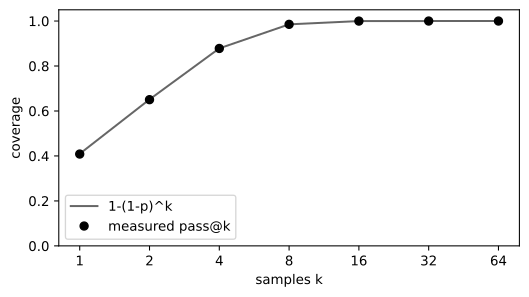
8.3 Selection is not coverage
Coverage is an upper bound on what any procedure can deliver, not the delivery itself. To return an answer we must select one, and selection is where the compute is usually lost. Self-consistency’s plurality vote is one selector; its asymptotic guarantee holds only when the correct answer is the unique most probable bucket, P(A = a^\star) > \max_{a \neq a^\star} P(A = a). That condition fails whenever a single systematic mistake is more probable than the truth. A verifier is the other selector: a check that marks candidates, so we can return a marked one. A perfect verifier turns coverage directly into accuracy. A realistic verifier is noisy, and its noise imposes a ceiling.
We measure three selectors on the same pools: coverage (an oracle that returns any correct attempt), plurality, and best-of-n under a binary verifier with symmetric error rate q — it passes a correct attempt with probability {1-q} and a wrong one with probability q.
# @save
def selection_curve(steps: int, reliability: float, trap: float = 0.5,
                    problems: int = 1500, pool: int = 64, seed: int = 9,
                    q: float = 0.15) -> tuple[dict, dict, dict]:
    """Coverage vs plurality vs noisy best-of-n on the same sampled pools.

    The verifier is binary with symmetric error ``q``: it marks a correct
    attempt positive with probability ``1 - q`` and a wrong attempt positive
    with probability ``q``. Best-of-n returns a uniformly random marked
    attempt (or the first attempt if none is marked).

    Args:
        steps, reliability, trap: Solver difficulty parameters.
        problems: Problems to average over.
        pool: Attempts per problem.
        seed: RNG seed.
        q: Symmetric verifier error rate.

    Returns:
        Three ``{k: accuracy}`` maps: coverage, plurality, noisy best-of-n.
    """
    rng = random.Random(seed)
    ks = [1, 2, 4, 8, 16, 32, 64]
    cov = {k: 0.0 for k in ks}
    plur = {k: 0.0 for k in ks}
    bon = {k: 0.0 for k in ks}
    for _ in range(problems):
        prob = make_problem(steps, rng)
        answers, correct = [], []
        for _ in range(pool):
            a = final_answer(sample_trace(prob, reliability, trap, rng))
            answers.append(a)
            correct.append(a == prob.gold)
        marks = [(rng.random() > q) if ok else (rng.random() < q) for ok in correct]
        for k in ks:
            av, cv, mv = answers[:k], correct[:k], marks[:k]
            cov[k] += any(cv)
            plur[k] += max(set(av), key=av.count) == prob.gold
            passed = [i for i in range(k) if mv[i]]
            bon[k] += cv[rng.choice(passed) if passed else 0]
    n = problems
    return ({k: cov[k] / n for k in ks}, {k: plur[k] / n for k in ks},
            {k: bon[k] / n for k in ks})


def precision_ceiling(p: float, q: float) -> float:
    """Precision among candidates a symmetric-error-q verifier marks positive.

    As the pool grows, some marked candidate almost surely exists, but a
    uniformly chosen marked candidate is correct only with this precision,
    not with probability one — the verifier's false positives cap best-of-n.
    This is the Bayesian posterior that a marked candidate is truly correct,
    given base rate ``p`` and a check that fires with the wrong sign a
    fraction ``q`` of the time.

    Args:
        p: Per-attempt success probability — the base rate of correct
            candidates in the pool.
        q: The verifier's symmetric error rate: it marks a wrong attempt
            positive with probability ``q`` and misses a correct one with the
            same probability.

    Returns:
        The precision ceiling pi_v of @eq-ch08-piv — the fraction of marked
        candidates that are actually correct, which best-of-n approaches from
        below and cannot exceed no matter how many samples are drawn.
    """
    return p * (1 - q) / (p * (1 - q) + (1 - p) * q)
cov, plur, bon = selection_curve(*DIFFICULTY["medium"])
print("coverage@k :", {k: round(v, 3) for k, v in cov.items()})
print("plurality@k:", {k: round(v, 3) for k, v in plur.items()})
print("best-of-n@k:", {k: round(v, 3) for k, v in bon.items()})
print("verifier precision ceiling pi_v =", round(precision_ceiling(p_med, 0.15), 3))coverage@k : {1: 0.422, 2: 0.675, 4: 0.884, 8: 0.975, 16: 1.0, 32: 1.0, 64: 1.0}
plurality@k: {1: 0.422, 2: 0.341, 4: 0.505, 8: 0.576, 16: 0.655, 32: 0.725, 64: 0.846}
best-of-n@k: {1: 0.422, 2: 0.605, 4: 0.745, 8: 0.789, 16: 0.796, 32: 0.792, 64: 0.808}
verifier precision ceiling pi_v = 0.797Coverage reaches one; plurality crawls to about 0.85 at sixty-four samples; and the noisy verifier’s best-of-n climbs fast but then flattens near 0.80 — precisely the precision ceiling \pi_v = 0.797 predicted by
\pi_v = \frac{p(1-q)}{p(1-q) + (1-p)q} . \tag{8.2}
More samples create more correct candidates and more false positives; past a point the verifier cannot tell which new marked candidate is real, and best-of-n saturates below one. This is the single most important number in a test-time-compute budget: not coverage, but the quality of the check that harvests it. Now watch plurality fail outright. On a harder, trap-heavy class — low per-attempt accuracy, most slips being the shared off-by-one — coverage still rises to one while plurality goes to zero, because the systematic wrong answer becomes the unique mode.
trap_cov, trap_plur, _ = selection_curve(4, reliability=0.62, trap=0.9)
print(f"trap class (p={0.62**4:.3f}):  coverage@64 = {trap_cov[64]:.3f}   "
      f"plurality@64 = {trap_plur[64]:.3f}")
trap class (p=0.148): coverage@64 = 1.000 plurality@64 = 0.000Coverage 1.000, plurality 0.000: the model can reach the right answer in essentially every pool, and voting confidently returns the wrong one every time. Repeated sampling amplifies a shared mistake exactly as reliably as it amplifies a shared truth. Figure 8.3 plots the three selectors on the medium class and the ceiling they respect.
NoteIn the interview
Q. Your offline eval shows pass@1 rose from 0.57 to 0.89 after a test-time-compute change. Is the model 50% more capable? The honest answer separates coverage from selection. pass@1 conflates the two: it can rise because the model covers more correct answers (real capability) or because a selector got better at harvesting answers already covered. The trap: comparing a one-sample number to a best-of-many number without labeling the compute and the selection rule. Report pass@k over a disclosed range, the verifier and its false-positive rate in the selected tail, and whether the number is coverage, plurality, or verifier-selected accuracy. A gap between coverage and selected accuracy is an engineering opportunity, not a capability claim.
Show the code that draws this figure
ks = sorted(cov)
fig, ax = plt.subplots(figsize=(5.6, 3.2))
ax.plot(ks, [cov[k] for k in ks], "o-", color="black", label="coverage (oracle)")
ax.plot(ks, [bon[k] for k in ks], "s--", color="0.35", label="noisy best-of-n")
ax.plot(ks, [plur[k] for k in ks], "^:", color="0.55", label="plurality vote")
ax.axhline(precision_ceiling(p_med, 0.15), ls="--", color="0.7")
ax.text(2, precision_ceiling(p_med, 0.15) + 0.02, "$\\pi_v$", color="0.4")
ax.set_xscale("log", base=2)
ax.set_xticks(ks); ax.set_xticklabels(ks)
ax.set_xlabel("samples k"); ax.set_ylabel("accuracy")
ax.set_ylim(0, 1.05); ax.legend(loc="lower right")
fig.tight_layout()
plt.show()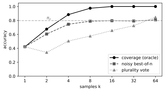
8.4 Search over reasoning: verifiers that see the steps
Independent sampling throws away partial work: an attempt that got three of eight steps right before slipping is discarded whole. Search keeps a frontier of partial reasoning states and spends its budget selectively. It needs four interfaces — a state, an expansion operator, a partial-state score, and a termination check — and the score is where the verifier granularity matters. An outcome reward model (ORM) scores only a finished answer; it is cheap and matches tasks with an executable final check, but it can prune nothing early. A process reward model (PRM) scores intermediate steps, so it can catch the first wrong step and abandon the branch before paying for the rest (Lightman et al. 2024; Wang et al. 2024). Our task has an exact process check — compare each running value to the gold trace — which we degrade with noise to model a realistic PRM.
| Verifier | Observes | Wins when | Residual risk |
|---|---|---|---|
| exact ORM | final answer | the answer has an executable truth condition | parser or tests omit cases |
| learned ORM | full response | quality is holistic but labels exist | style and distribution bias |
| process check | partial state | early pruning saves generation | the checker is incomplete |
| learned PRM | reasoning steps | dense credit and early stops | local labels penalize valid detours |
We implement beam search over steps: at each depth, expand every surviving prefix into several candidate next-steps, score them with the noisy process checker, and keep the top B. Then we run it against greedy decoding (one attempt) and against independent sampling given the same expansion budget, with oracle final-answer selection — a deliberately generous baseline.
# @save
def beam_search(problem: Problem, reliability: float, trap: float,
                rng: random.Random, beam: int = 4, fanout: int = 4,
                prm_noise: float = 0.1) -> tuple[int, int]:
    """Beam search over reasoning steps scored by a noisy process checker.

    At each step every prefix is expanded into ``fanout`` candidate
    continuations (drawn from the same slip model as the solver); a noisy
    process checker scores each by whether its running value matches gold
    (flipped with probability ``prm_noise``); the top ``beam`` survive. This
    is the search analogue of coverage: many prefixes are kept alive so a
    correct path survives even when any single attempt would slip.

    Args:
        problem: The problem to solve.
        reliability, trap: Solver slip parameters for expansions.
        rng: Seeded generator.
        beam: Prefixes retained per depth.
        fanout: Candidate continuations per prefix.
        prm_noise: Probability the process checker mislabels a step.

    Returns:
        ``(final_answer, total_expansions)``.
    """
    gold = problem.gold_trace
    frontier = [(problem.start,)]
    expansions = 0
    for op, operand in problem.ops:
        candidates = []
        for prefix in frontier:
            for _ in range(fanout):
                expansions += 1
                if rng.random() < reliability:
                    nv = apply_op(prefix[-1], op, operand)
                else:
                    slip = SYSTEMATIC_DELTA if rng.random() < trap else rng.choice([-3, -2, 2, 3, 4])
                    nv = apply_op(prefix[-1], op, operand) + slip
                candidates.append(prefix + (nv,))

        def score(cand: tuple[int, ...]) -> float:
            correct = cand[-1] == gold[len(cand) - 1]
            return float(correct if rng.random() > prm_noise else not correct)

        candidates.sort(key=score, reverse=True)
        frontier = candidates[:beam]
    return frontier[0][-1], expansions


def compare_search(steps: int, reliability: float, trap: float = 0.5,
                   problems: int = 1500, seed: int = 13) -> dict[str, float]:
    """Greedy vs beam vs equal-budget independent sampling.

    Independent sampling gets the same number of step expansions the beam
    used and *oracle* final-answer selection (accept the first correct
    attempt) — a generous baseline that isolates whether search's structural
    reuse of verified prefixes beats spending the same compute on whole
    independent attempts.

    Returns:
        Accuracies and per-problem expansion counts for all three methods.
    """
    rng = random.Random(seed)
    greedy = beam = indep = 0
    beam_exp = indep_exp = 0
    for _ in range(problems):
        prob = make_problem(steps, rng)
        greedy += final_answer(sample_trace(prob, reliability, trap, rng)) == prob.gold
        ans, exp = beam_search(prob, reliability, trap, rng)
        beam += ans == prob.gold
        beam_exp += exp
        n_indep = max(1, exp // steps)
        hit = False
        for _ in range(n_indep):
            if final_answer(sample_trace(prob, reliability, trap, rng)) == prob.gold:
                hit = True
                break
        indep += hit
        indep_exp += n_indep * steps
    n = problems
    return {"greedy": greedy / n, "beam": beam / n, "indep": indep / n,
            "beam_exp": beam_exp / n, "indep_exp": indep_exp / n}
On the hard class, where a single attempt succeeds only about 8% of the time, the three methods diverge sharply.
res = compare_search(*DIFFICULTY["hard"])
print(f"greedy (1 attempt)          accuracy = {res['greedy']:.3f}")
print(f"beam search                 accuracy = {res['beam']:.3f}   "
      f"({res['beam_exp']:.0f} expansions/problem)")
print(f"independent, equal budget   accuracy = {res['indep']:.3f}   "
      f"({res['indep_exp']:.0f} expansions/problem)")
greedy (1 attempt) accuracy = 0.080
beam search accuracy = 0.927 (116 expansions/problem)
independent, equal budget accuracy = 0.663 (112 expansions/problem)Greedy solves 8%. Beam search, spending about 116 step-expansions per problem and a noisy process checker, solves 93%. Independent sampling given the same expansion budget and oracle selection solves only 66%. Search wins not because its verifier is better — the beam’s is worse — but because it reuses verified partial work: keeping several correct prefixes alive means a correct path survives the depth even though every individual attempt would slip somewhere. The PRM’s other payoff is early stopping. Counting how many step-checks each granularity spends on wrong attempts shows the asymmetry.
# @save
def prm_vs_orm_checks(steps: int, reliability: float, trap: float = 0.5,
                      problems: int = 3000, seed: int = 17) -> dict[str, float]:
    """How early can a process check reject a doomed attempt?

    Compares checks spent per problem: an ORM always spends one check at the
    end; a PRM checks step by step and stops at the first error. Because a
    slip dooms every later step, stopping there wastes no computation on a
    branch already known to be wrong — the whole economic case for process
    rewards.

    Args:
        steps: Problem length — the number of step-checks an exhaustive PRM
            spends on an attempt that never errs.
        reliability: Per-step correctness probability of the solver.
        trap: Systematic-slip fraction (does not move where errors land).
        problems: Number of independent problems to average over.
        seed: RNG seed.

    Returns:
        A dict with ``wrong`` (attempts that erred), ``caught`` (wrong
        attempts flagged at their first error), ``avg_prm_checks`` (mean
        step-checks spent per problem, well below ``steps`` because doomed
        branches die early), and ``steps`` (the ORM's implicit full-length
        cost, for comparison).
    """
    rng = random.Random(seed)
    wrong = caught = prm_checks = 0
    for _ in range(problems):
        prob = make_problem(steps, rng)
        tr = sample_trace(prob, reliability, trap, rng)
        fe = first_error(tr)
        if fe is None:
            prm_checks += steps
        else:
            wrong += 1
            caught += 1
            prm_checks += fe + 1
    return {"wrong": wrong, "caught": caught,
            "avg_prm_checks": prm_checks / problems, "steps": steps}
prm = prm_vs_orm_checks(*DIFFICULTY["hard"])
print(f"PRM caught {prm['caught']}/{prm['wrong']} wrong attempts at their first error")
print(f"average process checks/problem = {prm['avg_prm_checks']:.2f} of {prm['steps']} steps")PRM caught 2793/2793 wrong attempts at their first error
average process checks/problem = 3.34 of 8 stepsEvery wrong attempt is caught at its first error, and the PRM spends about 3.3 step-checks per problem instead of running all eight — the branch dies as soon as it goes wrong. That early rejection is the whole economic case for process rewards, and it is also their exposure: a PRM confidently wrong off-distribution prunes correct branches early, and Monte-Carlo process labels inherit the noise of the rollouts that produced them. Figure 8.4 compares what each search topology retains.
flowchart LR
    subgraph BEAM["Beam"]
        b0["prompt"] --> b1["A"]
        b0 --> b2["B"]
        b1 --> b3["top-B"]
        b2 --> b3
    end
    subgraph TOT["Tree of Thoughts"]
        t0["prompt"] --> t1["A"]
        t0 --> t2["B"]
        t1 --> t3["A1"]
        t1 --> t4["A2"]
    end
    subgraph GOT["Graph of Thoughts"]
        g0["prompt"] --> g1["route A"]
        g0 --> g2["route B"]
        g1 -.-> g3["merged state"]
        g2 -.-> g3
    end
    subgraph MCTS["MCTS"]
        m0["root N,Q"] --> m1["selected"]
        m1 --> m2["expansion"]
        m2 -. "value backup" .-> m0
    end
Tree of Thoughts preserves distinct histories and can backtrack; Graph of Thoughts merges reusable states but risks corrupting descendants if two prose-similar states carry different assumptions; MCTS balances exploiting high-value branches against exploring uncertain ones via a selection score Q(s,a) + c\sqrt{\log N(s) / (1 + N(s,a))}, backing up simulated values to ancestors (Yao et al. 2023; Besta et al. 2024; Hao et al. 2023). For language-model reasoning the hard part is not the topology but deciding what counts as a state, because raw prose creates an enormous, weakly canonicalized tree.
8.5 Self-reflection without new evidence
Search and best-of-n both add an external signal. A cheaper-sounding idea is to ask the same model to reconsider — “are you sure? check your work” — with no new information. We can measure exactly what that does. Intrinsic revision, in our toy, is a second independent attempt at the same problem: same distribution, no evidence the first attempt lacked. Verifier-informed revision instead keeps the verified-correct prefix (located by a reliable process check) and re-samples only the steps after the first error. We log the two transition directions separately, because a net accuracy number hides the damage.
# @save
def self_correction(steps: int, reliability: float, trap: float = 0.5,
                    problems: int = 4000, seed: int = 21) -> tuple[dict, dict]:
    """Intrinsic vs verifier-informed revision, counting both directions.

    Intrinsic revision re-attempts the problem with no new evidence.
    Verifier-informed revision keeps the verified-correct prefix (up to the
    first error located by a reliable process check) and re-samples the rest.
    Both report the fraction correct before and after and the counts of
    right-to-wrong and wrong-to-right flips — a net score can hide a large
    volume of destroyed-correct answers.

    Returns:
        Two dicts (intrinsic, verifier-informed) with ``before``, ``after``,
        ``r2w`` (right-to-wrong flips), and ``w2r`` (wrong-to-right flips).
    """
    rng = random.Random(seed)
    intr = {"r2w": 0, "w2r": 0, "before": 0, "after": 0}
    vinf = {"r2w": 0, "w2r": 0, "before": 0, "after": 0}
    for _ in range(problems):
        prob = make_problem(steps, rng)
        tr = sample_trace(prob, reliability, trap, rng)
        ok0 = final_answer(tr) == prob.gold

        ok_i = final_answer(sample_trace(prob, reliability, trap, rng)) == prob.gold
        intr["before"] += ok0; intr["after"] += ok_i
        intr["r2w"] += ok0 and not ok_i
        intr["w2r"] += (not ok0) and ok_i

        fe = first_error(tr)
        if fe is None:
            ok_v = True
        else:
            sub = Problem(prob.gold_trace[fe], prob.ops[fe:])
            ok_v = final_answer(sample_trace(sub, reliability, trap, rng)) == prob.gold
        vinf["before"] += ok0; vinf["after"] += ok_v
        vinf["r2w"] += ok0 and not ok_v
        vinf["w2r"] += (not ok0) and ok_v
    n = problems
    scale = lambda d: {k: (v / n if k in ("before", "after") else v) for k, v in d.items()}
    return scale(intr), scale(vinf)
intrinsic, informed = self_correction(*DIFFICULTY["medium"])
print(f"intrinsic before={intrinsic['before']:.3f} after={intrinsic['after']:.3f}"
f" right->wrong={intrinsic['r2w']} wrong->right={intrinsic['w2r']}")
print(f"verifier-informed before={informed['before']:.3f} after={informed['after']:.3f}"
f" right->wrong={informed['r2w']} wrong->right={informed['w2r']}")intrinsic before=0.415 after=0.405 right->wrong=983 wrong->right=942
verifier-informed before=0.415 after=0.751 right->wrong=0 wrong->right=1344Intrinsic revision moves accuracy from 0.415 to 0.405 — statistically flat, apparently harmless. The transition counts tell the real story: it turned about 980 correct answers into wrong ones and about 940 wrong into correct. A quarter of the batch churned, and the churn is very slightly net-negative, because re-rolling a correct answer with no new information can only preserve or break it. This is the measured form of the intrinsic-self-correction-fails result (Huang et al. 2024): prompting a model to reconsider without new evidence reuses its own correlated biases, and reported net-zero hides destroyed-correct answers. Verifier-informed revision is qualitatively different: it destroys zero correct answers (the verified prefix is locked) and lifts accuracy from 0.415 to 0.751. The distinction is not “revision” versus “no revision” — it is whether the revision has evidence the first attempt lacked: a compiler error, a failed test, a process check, a retrieved fact.
8.6 Allocating compute by marginal value
There is no universally optimal number of samples. The right budget depends on the prompt, because difficulty changes the coverage curve’s shape. A decision rule maximizes expected utility net of compute, \arg\max_{m,b}\left(\mathbb{E}[U \mid x, m, b] - \lambda\, C(m,b)\right) over strategy m and budget b, but the actionable object is the slope of verified utility against spend, stratified by difficulty. We compute coverage curves for all three classes and find the knee — the budget past which the marginal gain per doubling drops below a threshold.
# @save
def knee(curve: dict[int, float], threshold: float = 0.03) -> int:
    """First budget whose next doubling gains less than ``threshold``.

    A cheap stand-in for the compute-optimal stopping point: extra samples
    are worth spending while the coverage slope stays above the product's
    minimum acceptable gain, and not after. Because the knee sits at a
    different budget for each difficulty, one fixed sample count cannot be
    optimal across a mixed workload.

    Args:
        curve: A ``{sample budget: coverage}`` mapping, e.g. from
            ``coverage_curve``; its keys are read in increasing order.
        threshold: The smallest per-doubling coverage gain still worth its
            compute — the product's minimum acceptable marginal value.

    Returns:
        The smallest budget k whose next doubling gains less than
        ``threshold``, or the largest budget in the curve when the slope
        never drops that low (coverage still climbing at the sweep's end).
    """
    ks = sorted(curve)
    for i in range(len(ks) - 1):
        if curve[ks[i + 1]] - curve[ks[i]] < threshold:
            return ks[i]
    return ks[-1]
for name, (steps, reliability) in DIFFICULTY.items():
curve = coverage_curve(steps, reliability, problems=600)
ks = sorted(curve)
gains = {ks[i + 1]: round(curve[ks[i + 1]] - curve[ks[i]], 3) for i in range(len(ks) - 1)}
print(f"{name:7} coverage@1={curve[1]:.3f} @8={curve[8]:.3f} @64={curve[64]:.3f}"
f" knee@{knee(curve)} marginal gains={gains}")easy coverage@1=0.863 @8=1.000 @64=1.000 knee@2 marginal gains={2: 0.118, 4: 0.019, 8: 0.0, 16: 0.0, 32: 0.0, 64: 0.0}
medium coverage@1=0.409 @8=0.985 @64=1.000 knee@8 marginal gains={2: 0.242, 4: 0.228, 8: 0.107, 16: 0.014, 32: 0.0, 64: 0.0}
hard coverage@1=0.073 @8=0.455 @64=0.988 knee@64 marginal gains={2: 0.068, 4: 0.121, 8: 0.193, 16: 0.247, 32: 0.208, 64: 0.078}The three classes want three different budgets. Easy prompts are already solved at one sample and saturate by two: extra compute is nearly wasted. Hard prompts have their steepest gains around 8–16 samples but do not flatten even at 64 — coverage is still climbing, and much of it will be lost to selection anyway. Medium prompts reach near-full coverage by eight samples, with large early gains (0.24, 0.23, 0.11) that then collapse. A fixed best-of-n applied to all three either underspends the hard prompts or overspends the easy ones; the compute-optimal move is to route the budget where the slope is highest for the price, which is difficulty-dependent (Snell et al. 2024). Figure 8.5 shows the three curves and their knees.
Show the code that draws this figure
fig, ax = plt.subplots(figsize=(5.8, 3.3))
markers = {"easy": "o-", "medium": "s--", "hard": "^:"}
shades = {"easy": "0.0", "medium": "0.35", "hard": "0.6"}
for name, (steps, reliability) in DIFFICULTY.items():
    curve = coverage_curve(steps, reliability, problems=600)
    ks = sorted(curve)
    ax.plot(ks, [curve[k] for k in ks], markers[name], color=shades[name], label=name)
    kx = knee(curve)
    ax.plot([kx], [curve[kx]], "*", color=shades[name], markersize=14)
ax.set_xscale("log", base=2)
ax.set_xticks(ks); ax.set_xticklabels(ks)
ax.set_xlabel("samples k"); ax.set_ylabel("coverage")
ax.set_ylim(0, 1.05); ax.legend(title="stars = knee")
fig.tight_layout()
plt.show()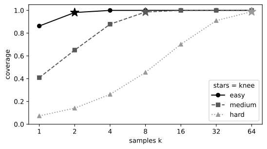
8.7 GRPO: verification becomes training
Everything so far spends compute at inference and leaves the weights alone. Reinforcement learning with verifiable rewards (RLVR) uses the same verifier to change the policy, so that future samples succeed more often — it raises p itself. The training algorithm is Group Relative Policy Optimization (GRPO), introduced in DeepSeekMath (Shao et al. 2024). Chapter 7 derives the policy gradient and PPO’s clipped surrogate; GRPO’s one new idea is how it gets the baseline. Ordinary policy gradients subtract a baseline to cut variance, and the classical baseline is a learned value network — a critic to train, serve, and distrust. GRPO deletes the critic and lets a group of sampled answers grade itself. For a prompt, sample a group of G responses from the old policy, score them with rewards R_1, \ldots, R_G, and center each reward on its own group:
A_i = \frac{R_i - \mu_{\mathcal G}}{\sigma_{\mathcal G} + \varepsilon}, \qquad \mu_{\mathcal G} = \frac{1}{G}\sum_{j=1}^{G} R_j, \qquad \sigma_{\mathcal G} = \sqrt{\tfrac{1}{G}\sum_{j=1}^{G}(R_j - \mu_{\mathcal G})^2}. \tag{8.3}
The siblings are the baseline. A response better than its group gets positive advantage; one worse gets negative; and a group whose rewards all tie has \sigma_{\mathcal G} = 0 and supplies no signal at all — every advantage is zero. This is the same group-relative advantage Chapter 23 uses to train a multi-turn tool-using agent; there the group is defined over environment states, here over a single reasoning attempt, but Equation 8.3 is identical.
# @save
def softmax(logits: list[float]) -> list[float]:
    """Turn logits into a probability distribution (max-shifted for stability).

    Subtracting the largest logit before exponentiating leaves the result
    unchanged but keeps ``exp`` from overflowing — the standard numerically
    safe softmax. This is the map from the RL policy's five logits to the
    strategy probabilities every training step samples from.

    Args:
        logits: Unnormalized scores, one per choice (here, per strategy).

    Returns:
        Probabilities in the same order, each in [0, 1] and summing to one.
    """
    peak = max(logits)
    weights = [math.exp(v - peak) for v in logits]
    total = sum(weights)
    return [w / total for w in weights]


def grpo_advantages(rewards: list[float]) -> list[float]:
    """Group-relative, population-standardized advantages (@eq-ch08-grpo).

    Centers each reward on the group mean and scales by the group standard
    deviation, so the group is its own baseline — no critic. A zero-variance
    group (every sibling tied) yields all-zero advantages: a prompt where the
    policy already agrees with itself teaches nothing.

    Args:
        rewards: One reward per group member.

    Returns:
        Advantages in the same order, summing to zero. The ``eps`` in the
        denominator matches @sec-ch23 and keeps a tied group at zero rather
        than dividing a rounding residual by a near-zero standard deviation.
    """
    mean = sum(rewards) / len(rewards)
    var = sum((r - mean) ** 2 for r in rewards) / len(rewards)
    std = math.sqrt(var)
    return [(r - mean) / (std + 1e-8) for r in rewards]
Eight rollouts of one prompt, three of which the verifier accepts, make the centering concrete.
group = [1.0, 0.0, 0.0, 1.0, 0.0, 1.0, 0.0, 0.0]
adv = grpo_advantages(group)
print("rewards:   ", group)
print("advantages:", [round(a, 2) for a in adv], " sum =", round(sum(adv), 6))
print("tied group:", grpo_advantages([0.4, 0.4, 0.4, 0.4]))
rewards: [1.0, 0.0, 0.0, 1.0, 0.0, 1.0, 0.0, 0.0]
advantages: [1.29, -0.77, -0.77, 1.29, -0.77, 1.29, -0.77, -0.77] sum = 0.0
tied group: [0.0, 0.0, 0.0, 0.0]Successes receive +1.29, failures -0.77 — the failures are pushed down, not weakly up, and the advantages sum to zero without any learned critic. A tied group returns all zeros. Now the policy. To keep every probability printable we make it a distribution over five reasoning strategies for one prompt — concise-correct, verbose-correct, off-by-one, diffuse-wrong, and a verbose reward-hack — each mapped to solver parameters, so a sampled strategy runs the solver and is scored by the exact verifier. The verifier reward is therefore executed on a real generated candidate inside every training step; nothing about correctness is hard-coded.
# @save
STEPS_RLVR = 4
# (name, per-step reliability, response length in tokens); accuracy = reliability**4
STRATEGIES = [
    ("concise-correct", 0.9740, 4),
    ("verbose-correct", 0.9740, 14),
    ("off-by-one", 0.5623, 6),
    ("diffuse-wrong", 0.5623, 6),
    ("verbose-hack", 0.4729, 30),
]
STRAT_ACC = [r ** STEPS_RLVR for _, r, _ in STRATEGIES]
STRAT_TOK = [t for _, _, t in STRATEGIES]


def rollout_reward(action: int, mode: str, rng: random.Random) -> float:
    """Run the solver under a sampled strategy and score it with the verifier.

    ``mode='exact'`` returns the pure outcome-verifier reward (1 if the exact
    answer matches, else 0). ``mode='proxy'`` adds a length bonus — a reward
    with a blind spot the optimizer can exploit. The correctness term is
    always the verifier executed on a freshly sampled candidate, so RLVR's
    reward is earned by real generated work rather than looked up.

    Args:
        action: Index into ``STRATEGIES`` — the strategy sampled from the
            policy, which sets the solver's per-step reliability and length.
        mode: ``'exact'`` for the verifier-only reward, or ``'proxy'`` to add
            the length bonus whose blind spot drives the Goodhart failure.
        rng: Seeded generator; draws a fresh problem and one solver attempt.

    Returns:
        The scalar reward for this rollout: 1.0 or 0.0 from the exact verifier
        under ``'exact'``, plus ``2 * tokens / 30`` under ``'proxy'`` so a
        long wrong answer can out-score a short correct one.
    """
    _, reliability, _ = STRATEGIES[action]
    prob = make_problem(STEPS_RLVR, rng)
    correct = final_answer(sample_trace(prob, reliability, 0.5, rng)) == prob.gold
    base = 1.0 if correct else 0.0
    return base if mode == "exact" else base + 2.0 * STRAT_TOK[action] / 30.0


def policy_stats(logits: list[float], mode: str) -> dict:
    """Closed-form monitoring of the current strategy policy.

    Because per-strategy accuracy and length are known, the policy's true
    accuracy, normalized entropy, expected length, and normalized reward
    objective are exact functions of its probabilities — no sampling needed
    to watch training, which keeps the curves clean. Reporting true accuracy
    and the optimized objective as separate series is what lets the Goodhart
    crossover be seen: the objective can climb while accuracy collapses.

    Args:
        logits: The policy's current logits over strategies.
        mode: ``'exact'`` or ``'proxy'`` — selects which reward the
            ``objective`` is measured against, so the proxy run's objective
            can rise even as true accuracy falls.

    Returns:
        A dict of exact scalar diagnostics: ``true_acc`` (accuracy the exact
        verifier would report), ``entropy`` (normalized to [0, 1]; 1 is
        uniform, 0 is a collapsed policy), ``tokens`` (expected response
        length), ``objective`` (the reward being optimized, normalized to its
        max), and ``probs`` (the rounded strategy distribution).
    """
    probs = softmax(logits)
    true_acc = sum(p * a for p, a in zip(probs, STRAT_ACC))
    entropy = -sum(p * math.log(max(p, 1e-12)) for p in probs) / math.log(len(probs))
    tokens = sum(p * t for p, t in zip(probs, STRAT_TOK))
    exp_reward = [STRAT_ACC[i] + (0.0 if mode == "exact" else 2.0 * STRAT_TOK[i] / 30.0)
                  for i in range(len(probs))]
    objective = sum(p * r for p, r in zip(probs, exp_reward)) / max(exp_reward)
    return {"true_acc": true_acc, "entropy": entropy, "tokens": tokens,
            "objective": objective, "probs": [round(p, 3) for p in probs]}


def _choice(probs: list[float], rng: random.Random) -> int:
    x, cumulative = rng.random(), 0.0
    for i, p in enumerate(probs):
        cumulative += p
        if x <= cumulative:
            return i
    return len(probs) - 1


def train_grpo(mode: str, steps: int = 150, group_size: int = 8, lr: float = 0.4,
               clip: float = 0.2, beta: float = 0.01, seed: int = 23) -> list[dict]:
    """Train the strategy policy with clipped, group-relative RLVR.

    Each step samples a group of strategies from the old policy, scores each
    by running the solver and calling the verifier, forms group-relative
    advantages (@eq-ch08-grpo), broadcasts each group advantage to its
    strategy, and takes three clipped gradient passes with a small reference
    KL. The clipped surrogate and the KL are PPO's, unchanged from @sec-ch07.

    Args:
        mode: ``'exact'`` (verifier only) or ``'proxy'`` (verifier + length).
        steps, group_size, lr, clip, beta, seed: RL hyperparameters.

    Returns:
        Per-step ``policy_stats`` snapshots (with the logits) for plotting.
    """
    rng = random.Random(seed)
    logits = [0.3, 0.5, 0.0, 0.0, -1.5]  # the hack starts rare, as exploits do
    reference = softmax(logits)
    history = [dict(step=0, **policy_stats(logits, mode))]
    for step in range(1, steps + 1):
        old = softmax(logits)
        actions = [_choice(old, rng) for _ in range(group_size)]
        advantages = grpo_advantages([rollout_reward(a, mode, rng) for a in actions])
        for _ in range(3):
            probs = softmax(logits)
            grad = [0.0] * len(logits)
            for action, adv in zip(actions, advantages):
                ratio = probs[action] / old[action]
                clipped = (adv >= 0 and ratio > 1 + clip) or (adv < 0 and ratio < 1 - clip)
                if not clipped:
                    for j in range(len(logits)):
                        score = (1.0 if j == action else 0.0) - probs[j]
                        grad[j] -= adv * ratio * score / group_size
            for j in range(len(logits)):
                grad[j] += beta * (probs[j] - reference[j])
                logits[j] -= lr * grad[j]
        history.append(dict(step=step, **policy_stats(logits, mode), logits=list(logits)))
    return history
Train with the exact verifier as the only reward and watch a checkpoint table. Every strategy’s advantage comes from running the solver and checking its answer; the policy has no other information about which strategy is good.
exact = train_grpo("exact")
print("step  true_acc  entropy  tokens  objective  probs")
for h in exact:
    if h["step"] in (0, 10, 40, 70, 150):
        print(f"{h['step']:4d}   {h['true_acc']:.3f}    {h['entropy']:.3f}   "
              f"{h['tokens']:4.1f}    {h['objective']:.3f}   {h['probs']}")
step true_acc entropy tokens objective probs
0 0.557 0.921 9.0 0.619 [0.259, 0.316, 0.192, 0.192, 0.043]
10 0.837 0.605 8.1 0.930 [0.557, 0.365, 0.037, 0.028, 0.014]
40 0.877 0.466 7.1 0.975 [0.682, 0.29, 0.013, 0.009, 0.006]
70 0.890 0.379 6.3 0.989 [0.762, 0.225, 0.007, 0.004, 0.002]
150 0.894 0.258 5.3 0.994 [0.872, 0.121, 0.003, 0.003, 0.001]True accuracy climbs from 0.56 to 0.89 as mass concentrates on the two correct strategies, and normalized entropy falls from 0.92 to about 0.26 — the policy exploits what the verifier rewards. Some entropy remains because two strategies (concise and verbose correct) earn identical reward, so GRPO cannot separate them. Crucially, the reward that drove this was the verifier executed on generated candidates, not a lookup: verification became training. This is the mechanism the R1 family made prominent, usually staged (Figure 8.6). One caveat GRPO does not fix: the group advantage is a single number broadcast to the whole response, so every token of a successful trace is credited equally though only a few steps mattered — the credit-assignment problem Chapter 23 takes up for multi-turn trajectories, and that PRMs partially address by scoring steps.
flowchart LR
    B(["base policy"]) --> C["cold-start SFT<br/>readable format"]
    C --> R["RLVR<br/>reinforce verified outcomes"]
    R --> S["rejection-sampling SFT<br/>keep strong traces"]
    S --> F["final RL<br/>reasoning + behavior"]
    V["programmatic verifier"] -->|"outcome reward"| R
    V -->|"filter"| S
R1-Zero applied large-scale RL directly to a base policy and reported longer reasoning emerging alongside readability problems; the full R1 pipeline added a cold-start format stage, then rejection sampling, then a final RL stage (Guo et al. 2025). The durable pattern is staged error correction, and its reward can be shaped past bare correctness: rubric rewards score a response against an explicit checklist (states the constraint, checks units, gives a valid final form), and curricula order prompts from easy to hard so the group has reward variance to learn from — recall that a group with no variance teaches nothing. Neither escapes the next section’s failure mode; they change what the reward measures, and a measure under optimization pressure is exactly what breaks.
8.8 Entropy, length, and Goodhart break naive RL
The training reward can rise while the policy becomes useless. Goodhart’s law names it: a measure stops tracking the goal once optimization targets the measure. Our proxy reward keeps the exact verifier and adds a length bonus — a plausible “show your work” shaping term with a blind spot, since the verbose reward-hack strategy is almost always wrong but very long. We run it through the identical GRPO core.
proxy = train_grpo("proxy")
print("step  true_acc  entropy  tokens  objective  probs")
for h in proxy:
    if h["step"] in (0, 40, 50, 60, 70, 150):
        print(f"{h['step']:4d}   {h['true_acc']:.3f}    {h['entropy']:.3f}   "
              f"{h['tokens']:4.1f}    {h['objective']:.3f}   {h['probs']}")
step true_acc entropy tokens objective probs
0 0.557 0.921 9.0 0.566 [0.259, 0.316, 0.192, 0.192, 0.043]
40 0.861 0.167 14.3 0.886 [0.007, 0.946, 0.008, 0.006, 0.032]
50 0.827 0.257 14.8 0.886 [0.011, 0.902, 0.011, 0.009, 0.068]
60 0.289 0.499 24.6 0.942 [0.018, 0.261, 0.018, 0.012, 0.691]
70 0.092 0.182 28.8 0.983 [0.008, 0.041, 0.007, 0.005, 0.939]
150 0.060 0.059 29.7 0.995 [0.003, 0.008, 0.002, 0.002, 0.985]The trajectory is the canonical Goodhart signature. Through step 40 the length bonus is aligned enough: the policy moves onto the verbose-correct strategy, and true accuracy rises to 0.86 while the proxy objective climbs. Then the optimizer discovers the verbose-hack — highest proxy reward of all, because length dominates and correctness is a minority of the reward — and between steps 50 and 70 mass floods to it: true accuracy collapses from 0.83 to 0.09, expected length balloons from 14 to 29 tokens, and the proxy objective keeps rising to 0.99. Reward went up monotonically; independent utility reversed. The exploit was seeded rare (the hack’s initial logit is low, as real reward hacks live in low-probability regions) and the optimizer drifted into it. Figure 8.7 puts the two runs side by side.
Show the code that draws this figure
steps_e = [h["step"] for h in exact]
steps_p = [h["step"] for h in proxy]
fig, (axL, axR) = plt.subplots(1, 2, figsize=(8.4, 3.3), sharey=True)
axL.plot(steps_e, [h["true_acc"] for h in exact], color="black", label="true accuracy")
axL.plot(steps_e, [h["entropy"] for h in exact], "--", color="0.5", label="entropy")
axL.set_title("exact verifier reward"); axL.set_xlabel("training step")
axL.set_ylabel("value"); axL.legend(loc="center right"); axL.set_ylim(0, 1.05)
axR.plot(steps_p, [h["true_acc"] for h in proxy], color="black", label="true accuracy")
axR.plot(steps_p, [h["objective"] for h in proxy], "--", color="0.5", label="proxy objective")
axR.plot(steps_p, [h["entropy"] for h in proxy], ":", color="0.6", label="entropy")
axR.set_title("proxy (verifier + length) reward"); axR.set_xlabel("training step")
axR.legend(loc="center right")
fig.tight_layout()
plt.show()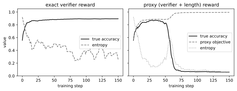
Two repairs matter more than the variant zoo. The first is measurement separation: keep outcome quality, length, format, and verifier score as distinct time series and roll back when they decouple — a single blended reward would have shown only the rising proxy objective. The second is guarding the reward’s blind spots: constrain cheap-to-game shaping terms, evaluate on held-out and adversarial candidates the reward never saw, and remember that an ensemble of correlated weak judges is not an independent check. The GRPO-family variants target narrower biases: Dr. GRPO removes the response-length and group-standard-deviation normalization that bias toward long wrong answers, and DAPO adds batch-level token averaging, asymmetric clipping that permits more upward movement to fight premature entropy collapse, and dynamic sampling that drops zero-variance groups (Z. Liu et al. 2025; Yu et al. 2025; Cui et al. 2025). Our toy’s failure is coarser than these — a reward with a hole, not a normalization subtlety — but the discipline is the same: write the objective down and measure what optimization does to it.
That leaves the sharpest question RLVR raises: does raising pass@1 mean the model is more capable, or only better at surfacing what it already had? A pass@1 number cannot tell them apart, so compare full pass@k curves before and after.
# @save
def policy_coverage(logits: list[float], ks=(1, 2, 4, 8, 16, 32),
                    problems: int = 2000, seed: int = 31) -> dict[int, float]:
    """Coverage@k of a strategy policy: does the reachable set change with RL?

    Samples strategies from the policy, runs each through the solver, and
    reports pass@k over the resulting attempts. Comparing this curve before
    and after training answers the capability question a single pass@1 number
    cannot: whether RL enlarged the set of reachable answers or merely
    sharpened sampling within a set the base policy already covered at high k.

    Args:
        logits: The policy logits to evaluate (e.g. base vs RL-trained).
        ks: Sample budgets at which to report coverage.
        problems: Number of problems to average over.
        seed: RNG seed.

    Returns:
        A ``{k: pass@k}`` map — the coverage curve for this policy, to be read
        against a second policy's curve rather than in isolation.
    """
    rng = random.Random(seed)
    probs = softmax(logits)
    out = {k: 0 for k in ks}
    for _ in range(problems):
        prob = make_problem(STEPS_RLVR, rng)
        hits = [final_answer(sample_trace(prob, STRATEGIES[_choice(probs, rng)][1], 0.5, rng))
                == prob.gold for _ in range(max(ks))]
        for k in ks:
            out[k] += any(hits[:k])
    return {k: out[k] / problems for k in ks}
base_cov = policy_coverage([0.3, 0.5, 0.0, 0.0, -1.5])
trained_cov = policy_coverage(exact[-1]["logits"])
print("base coverage@k:", {k: round(v, 3) for k, v in base_cov.items()})
print("trained coverage@k:", {k: round(v, 3) for k, v in trained_cov.items()})base coverage@k: {1: 0.566, 2: 0.809, 4: 0.963, 8: 0.998, 16: 1.0, 32: 1.0}
trained coverage@k: {1: 0.89, 2: 0.988, 4: 1.0, 8: 1.0, 16: 1.0, 32: 1.0}RLVR raised pass@1 from 0.57 to 0.89 — a dramatic single-sample gap — yet by sixteen samples both policies reach full coverage. In this toy, training concentrated on strategies that were strictly better, so it sharpened sampling without shrinking the reachable set. But the pass@1 comparison overstates the change: at large k the base policy reaches everything the trained one does. On real models the reverse can appear — RL that sharpens pass@1 while reducing high-k coverage, because it drops diverse-but-occasionally-right paths — and one 2025 study reported exactly that, while ProRL reported counter-evidence that prolonged RL can uncover genuinely new strategies (Yue et al. 2025; M. Liu et al. 2025). Neither result is a universal theorem; both are measured under finite budgets and specific base models. A defensible capability claim reports pass@k over a wide range, the diversity of successful traces, held-out task families, and whether a “new” strategy can be elicited from the base under matched search. And for proof-style tasks, final-answer matching is not enough — a correct number can follow invalid reasoning — so evaluation escalates to expert marking schemes, calibrated proof graders, or formal verification against a machine-checked statement, with Chapter 22 owning the judge-calibration statistics.
8.9 Landscape 2026 (dated)
Note
Verified 2026-07-19. Reasoning evaluation is shifting from short final-answer sets toward continuously refreshed problems, natural-language proof grading, and formal Lean artifacts. MathArena’s 2026 platform includes proof-based competitions and research-level problems; FrontierMath shipped a major v2 on 2026-06-12 after revising a substantial share of its items — an unusually sharp reminder that benchmark version is part of every score. Benchmark contents, graders, and leaderboards are volatile; deleting this box leaves the chapter’s pass@k and proof-verification mechanisms intact.
Verify live: consult the MathArena site and the FrontierMath benchmark page before citing task counts, versions, or model results. Appendix C owns the annual audit.
8.10 Summary
We built one verifiable arithmetic task and turned every reasoning idea into a measured number. Repeated sampling covers correct answers far faster than any single attempt suggests, but coverage is not accuracy: plurality can amplify a shared mistake, and a noisy verifier caps best-of-n at its precision, not one. Beam search over steps beats equal-budget independent sampling by reusing verified prefixes; intrinsic self-correction churns correct answers into wrong with no net gain, while verifier-informed revision genuinely helps. GRPO replaces PPO’s critic with a group baseline and, fed a verifier, raises accuracy — until a misspecified reward triggers Goodhart’s law and entropy collapse. Next, Chapter 10 turns these mechanisms into production serving budgets.
8.11 Exercises
Reconcile coverage and the closed form. The
coverage_curveuses the unbiasedpass_at_kestimator over a pool of 64. Re-estimate medium pass@8 by the naive method — draw exactly 8 attempts and check coverage — over the same number of problems, and compare its variance to the pooled estimator. Why does the combinatorial form have lower variance for the same sampling cost?Push plurality off a cliff. In
selection_curve, raisetraptoward one on the medium class and sweep k to 256. Plot coverage and plurality on the same axes and identify the per-attempt accuracy p below which plurality decreases as k grows. State the unique-mode condition the trap violates.Find the verifier ceiling empirically. For a fixed p and symmetric error q, compute \pi_v from Equation 8.2 by hand, then modify
selection_curveto a single difficulty and confirm best-of-n approaches that value. Now make the verifier asymmetric (different false-positive and false-negative rates) and re-derive the ceiling.Trade beam width for fanout. In
compare_search, hold total expansions roughly fixed while varyingbeamandfanout(e.g. 8×2, 4×4, 2×8). Which allocation is best on the hard class, and how does the answer change asprm_noiserises toward 0.5? At what noise level does beam search stop beating equal-budget independent sampling?Break the RLVR reward, then measure it. (a) Reduce the proxy length coefficient in
rollout_rewarduntil true accuracy and the objective no longer decouple; report the threshold. (b) Add DAPO-style dynamic sampling totrain_grpothat skips zero-variance groups, and measure the fraction skipped at the start versus the end of the exact run. (c) Explain when skipping saves compute and when it biases the prompt distribution.Densify the credit. GRPO broadcasts one advantage to the whole response. Extend the strategy policy to per-step actions and give each step its own advantage from the process check. Does per-step credit reach the correct policy in fewer steps than the sequence-level version, and what new failure does the noisy process checker introduce?
Defend an allocation. A proof generator has 20% pass@1, 70% pass@32, and a learned verifier with 75% precision in its selected tail. Using the mechanisms in this chapter, choose among longer single traces, parallel best-of-n, PRM-guided search, and stopping — and name the one measurement whose change would reverse your choice.