flowchart TD
    F(["Reproducible production failure"]) --> B["Freeze a baseline, reproduce it"]
    B --> Q{"What is actually missing?"}
    Q -->|"mutable facts, citations"| R["Retrieval / RAG — Chapter 14"]
    Q -->|"private or live state"| S["Authorized state read"]
    Q -->|"external effect"| T["Typed tool + policy"]
    Q -->|"ranking geometry"| E["Embedding / reranker tuning"]
    Q -->|"response behavior"| H{"Which supervision exists?"}
    H -->|"target responses"| SFT["SFT, via LoRA or full tuning"]
    H -->|"ranked pairs"| DPO["Preference tuning"]
    H -->|"reliable verifier"| RFT["Reinforcement fine-tuning"]
    Q -->|"teacher works, serving too costly"| KD["Distill to a smaller student"]
    Q -->|"compatible specialists exist"| M["Merge task vectors"]
    SFT --> G["Four-set task + regression gate"]
    DPO --> G
    RFT --> G
    KD --> G
    M --> G
    E --> G
    G -->|"pass"| P(["Canary, monitor, promote"])
    G -->|"fail"| B
11 Customization: distillation, merging, and fine-tuning
We are now ready to change a model’s weights on purpose, and to measure what each change costs. We take the tinygpt from Chapter 2 — a 100-thousand-parameter decoder that we will pretrain into a small generalist — and put it through the whole customization toolbox, in executed steps: (i) a decision that often ends in not touching the weights; (ii) LoRA, a low-rank update we bolt onto the frozen model and train on a new task, counting exactly how few parameters move; (iii) QLoRA, the same update over a four-bit base; (iv) distillation, moving a teacher’s behavior into a student four times smaller, where the teacher’s full distribution beats its hard labels; (v) merging, adding two task vectors and watching them interfere; (vi) catastrophic forgetting, which our own LoRA run causes, and the replay mix that repairs it; and (vii) a four-set release gate that ships one candidate and rejects another. The derivations of SFT and DPO belong to Chapter 7 and the quantization ladder to Chapter 10; this chapter is where those ingredients become a customization decision and a release workflow.
Everything runs on a CPU in under a minute. The tasks are synthetic character transforms on tagged four-digit strings, so a tiny model can learn them and we can read exact accuracies — but the mechanisms (the low-rank algebra, the NF4 codebook, the distillation loss, the task-vector merge, the gate) are the ones a seven-billion-parameter run uses. Only the constants change.
11.1 Deciding whether to change the weights
A support assistant keeps answering with last quarter’s refund policy. The team proposes fine-tuning, because the mistake appears in the model’s output. That is one layer too late. The policy changes every quarter, must be cited, and depends on the customer’s jurisdiction. Baking today’s answer into weights would make updates a training run, hide provenance, and make stale behavior hard to revoke. The failure is missing evidence, not missing behavior.
The first customization skill is deciding not to customize weights. Name the failing contract before choosing a method:
- Evidence — the answer needs facts that are private, changing, attributable, or too rare to trust to parametric recall. Retrieve them and require grounded use.
- State — the answer depends on an account, a workflow, or the current environment. Read state through an authorized interface.
- Effect — success means changing the world: issuing a refund, running code, updating a ticket. Use a typed tool with validation.
- Behavior — the information is present but the model picks the wrong format, tone, classification, or refusal. Prompting or post-training may fit.
- Representation — retrieval returns the wrong things because items are poorly embedded or ranked. Tune the retriever or reranker against judgments.
- Economics — a strong model works but is too slow or costly per query. Distill it into a smaller student, or route easy cases to one.
Only the last three are weight-side problems, and only behavior and economics are this chapter’s. The evidence branch — retrieval and RAG — is Chapter 14’s; when the missing mechanism is grounded facts, close this branch and go there. Figure 11.1 draws the escalation and its stop conditions; every weight-changing path returns to the same gate.
Once the defect is genuinely model behavior, the kind of supervision the team can produce selects the method — this table is the chapter’s spine, not a maturity ladder to climb.
| Supervision available | Most direct method | What it teaches |
|---|---|---|
| “here is the response to write” | SFT (often LoRA/QLoRA) | conditional imitation: input to target |
| “response A beats response B” | preference tuning (DPO) | relative choice under a prompt distribution |
| “this outcome scores 0.8” | reinforcement fine-tuning | search against a stable verifier |
| “here is the teacher’s distribution” | logit distillation | relative plausibility across alternatives |
| “here are the teacher’s completions” | sequence distillation | imitation of teacher trajectories |
| “these specialists share one base” | model merging | an evaluated combination of updates |
SFT is not an inferior RL; RFT is not useful when the grader is noisy. Pick the supervision that most directly expresses the contract. Two shortcuts fail this tree: fine-tuning on documents is not a database (memorization is uneven and updates need retraining), and fine-tuning on a handful of bad outputs is not a specification (it may encode one accidental wording). Diagnose the invariant, then collect supervision around it.
11.2 LoRA and QLoRA isolate a small trainable update
Everything below builds on one base model, so we fix determinism once and pull the tinygpt class straight out of Chapter 2’s tangled module rather than re-implementing it. Recall from Chapter 2 that TinyGPT is a decoder-only transformer with pre-norm blocks, SwiGLU feed-forward layers, and a tied LM head; we reuse it unchanged.
from __future__ import annotations
import torch
torch.set_num_threads(4)  # tiny models: fewer threads run faster and stay deterministic
torch.manual_seed(0)
<torch._C.Generator at 0x7f000002a9d0># @save
import copy
import importlib.util
import sys
from pathlib import Path
import numpy as np
import torch
from torch import nn, Tensor
from torch.nn import functional as F
def load_chapter_module(chapter: str, name: str):
"""Import a finished chapter's tangled module by path, not by install.
Earlier chapters tangle their teaching code into ``code/chNN/_generated.py``.
Rather than copy the Chapter 2 transformer, we walk up from the working
directory to the book root and load it under a chapter-unique module name.
Args:
chapter: The code directory to load, e.g. ``"ch02"``.
name: The module name to register it under.
Returns:
The executed module object.
"""
root = Path.cwd()
while not (root / "code" / chapter / "_generated.py").exists():
if root.parent == root:
raise FileNotFoundError(f"cannot find code/{chapter}/_generated.py")
root = root.parent
spec = importlib.util.spec_from_file_location(name, root / "code" / chapter / "_generated.py")
module = importlib.util.module_from_spec(spec)
sys.modules[name] = module
spec.loader.exec_module(module)
return module
_ch02 = load_chapter_module("ch02", "ch11_ch02")
TinyGPT, GPTConfig, generate = _ch02.TinyGPT, _ch02.GPTConfig, _ch02.generateThe task is a tagged transform. Each example is a one-character operation tag, four digits, =, and the four-digit answer, ended by |: A8012=9123| says “apply operation A (add one) to 8012.” The tag lets one model hold several operations at once, so forgetting and merging are about capacity and interference, not logical contradiction.
# @save
ALPHABET = "0123456789=|EAFS"
STOI = {c: i for i, c in enumerate(ALPHABET)}
VOCAB, NDIG, BLOCK, EQ = len(ALPHABET), 4, 24, STOI["="]

# echo, add-one, flip (nine's complement), and shift-by-position
OPS = {
    "E": lambda p: list(p),
    "A": lambda p: [(d + 1) % 10 for d in p],
    "F": lambda p: [9 - d for d in p],
    "S": lambda p: [(d + i) % 10 for i, d in enumerate(p)],
}


def make_example(rng: np.random.Generator, op: str) -> str:
    """Return one ``op<digits>=<answer>|`` example with random digits."""
    p = list(rng.integers(0, 10, size=NDIG))
    return op + "".join(map(str, p)) + "=" + "".join(map(str, OPS[op](p))) + "|"


def make_stream(ops, n: int, seed: int) -> Tensor:
    """Encode ``n`` examples of one or more operations into a token stream.

    Args:
        ops: A single operation tag or a list cycled across the examples.
        n: Number of examples to draw.
        seed: Seed for the digit generator, so a dataset is reproducible.

    Returns:
        A 1-D long tensor of token ids ready for windowed batching.
    """
    if isinstance(ops, str):
        ops = [ops]
    rng = np.random.default_rng(seed)
    text = "".join(make_example(rng, ops[i % len(ops)]) for i in range(n))
    return torch.tensor([STOI[c] for c in text], dtype=torch.long)
Training and evaluation are the standard character-LM loop from Chapter 2, wrapped so every later section can reuse them. fit runs AdamW with linear warmup and gradient clipping; accuracy generates the answer greedily and scores it per character, a smoother signal than exact-match at this scale.
# @save
def batch(stream: Tensor, size: int, gen: torch.Generator) -> tuple[Tensor, Tensor]:
    """Draw aligned (input, next-token) windows from a token stream.

    Args:
        stream: The 1-D token stream to sample from.
        size: Number of windows to draw.
        gen: Seeded generator choosing the window offsets.

    Returns:
        A tuple ``(inputs, targets)``, each shaped ``(size, BLOCK)``, with
        targets the inputs shifted one position later.
    """
    starts = torch.randint(0, stream.numel() - BLOCK - 1, (size,), generator=gen)
    x = torch.stack([stream[s:s + BLOCK] for s in starts])
    y = torch.stack([stream[s + 1:s + BLOCK + 1] for s in starts])
    return x, y


def fit(model, stream, steps, lr, size=64, seed=0, warmup=20):
    """Train a model (or its trainable subset) with warmup-then-flat AdamW.

    Only parameters with ``requires_grad`` receive updates, so the same loop
    trains a full model or just a set of LoRA matrices. Gradients are clipped
    to unit norm to keep the tiny model's steps stable.

    Args:
        model: Any module whose ``forward`` returns ``(logits, loss, cache)``.
        stream: The token stream to sample windows from.
        steps: Number of optimizer steps.
        lr: Peak learning rate after warmup.
        size: Batch size in windows.
        seed: Seed for the window sampler.
        warmup: Steps of linear warmup from zero to ``lr``.

    Returns:
        The list of per-step training losses.
    """
    params = [p for p in model.parameters() if p.requires_grad]
    opt = torch.optim.AdamW(params, lr=lr)
    gen = torch.Generator().manual_seed(seed)
    model.train()
    losses = []
    for step in range(steps):
        for group in opt.param_groups:
            group["lr"] = lr * min(1.0, (step + 1) / warmup)
        x, y = batch(stream, size, gen)
        opt.zero_grad(set_to_none=True)
        _, loss, _ = model(x, y)
        loss.backward()
        torch.nn.utils.clip_grad_norm_(params, 1.0)
        opt.step()
        losses.append(loss.item())
    return losses


@torch.no_grad()
def accuracy(model, op, n=150, seed=999):
    """Return the per-character answer accuracy of ``model`` on operation ``op``.

    For each of ``n`` fresh prompts the model greedily generates four answer
    characters, which are compared position-by-position against the true
    transform. A value near 0.1 is chance; 1.0 is a solved task.

    Args:
        model: The model to score.
        op: The operation tag to test.
        n: Number of held-out prompts.
        seed: Seed for the evaluation prompts, kept apart from training seeds.

    Returns:
        The fraction of answer characters generated correctly.
    """
    rng = np.random.default_rng(seed)
    model.eval()
    correct = total = 0
    for _ in range(n):
        p = list(rng.integers(0, 10, size=NDIG))
        prompt = op + "".join(map(str, p)) + "="
        ids = torch.tensor([[STOI[c] for c in prompt]])
        out = generate(model, ids, NDIG, temperature=0.0)
        got = [ALPHABET[i] for i in out[0, -NDIG:].tolist()]
        correct += sum(a == b for a, b in zip(got, map(str, OPS[op](p))))
        total += NDIG
    return correct / total


def small_gpt(d_model, n_layers, n_heads):
    """Build a fresh tinygpt over the tagged-transform vocabulary."""
    return TinyGPT(GPTConfig(vocab_size=VOCAB, block_size=BLOCK,
                             d_model=d_model, n_heads=n_heads, n_layers=n_layers))
We pretrain the base as a generalist on a fifty-fifty mix of echo (E) and add-one (A). These are its established capabilities — the ones a customization must not silently break.
torch.manual_seed(1)
base = small_gpt(d_model=64, n_layers=2, n_heads=4)
fit(base, make_stream(["E", "A"], 1200, seed=10), steps=500, lr=2e-3, seed=1)
base_caps = {op: accuracy(base, op) for op in "EAFS"}
print("base parameters:", sum(p.numel() for p in base.parameters()))
print("base capabilities:", {op: round(v, 2) for op, v in base_caps.items()})
base parameters: 101376
base capabilities: {'E': 1.0, 'A': 1.0, 'F': 0.06, 'S': 0.32}The base echoes and adds one perfectly (E and A at 1.00) and, as expected, has no idea how to flip (F) or shift (S) — those sit near chance. Now we teach it to flip, the customization task for the rest of the chapter.
Full fine-tuning lets every parameter move. That is right when a broad distribution shift needs capacity, but it couples one small task to the whole model’s optimizer state, checkpoint size, and serving cost. LoRA constrains the update instead (Hu et al. 2021). For a frozen weight matrix W_0 \in \mathbb{R}^{d_{out} \times d_{in}}, it learns
h = W_0 x + \frac{\alpha}{r}\, B A x, \qquad A \in \mathbb{R}^{r \times d_{in}},\ B \in \mathbb{R}^{d_{out} \times r}, \tag{11.1}
with rank r \ll \min(d_{in}, d_{out}) and a scale \alpha. The trainable count is r(d_{in} + d_{out}) instead of d_{in} d_{out} — the rank-r bottleneck is the whole idea. Initializing B = 0 makes the first forward pass identical to the base, so training starts from the model we trust. In code, a LoRA layer wraps an existing nn.Linear, freezes it, and adds the two small matrices.
# @save
class LoRALinear(nn.Module):
    """A frozen linear layer plus a trainable low-rank update ``(alpha/r)·B·A``.

    The wrapped layer's weights never receive gradients; only ``A`` and ``B``
    do. With ``B`` initialized to zero the layer starts as an exact copy of the
    base, so fine-tuning departs from trusted behavior rather than from noise.
    """

    def __init__(self, linear: nn.Linear, rank: int, alpha: float) -> None:
        super().__init__()
        self.linear = linear
        for p in self.linear.parameters():
            p.requires_grad_(False)
        out_features, in_features = linear.weight.shape
        self.scaling = alpha / rank
        self.A = nn.Parameter(torch.randn(rank, in_features) * 0.02)
        self.B = nn.Parameter(torch.zeros(out_features, rank))

    def forward(self, x: Tensor) -> Tensor:
        return self.linear(x) + self.scaling * (x @ self.A.t()) @ self.B.t()

    @property
    def delta(self) -> Tensor:
        """Return the realized dense update ``(alpha/r)·B·A`` for this layer."""
        return self.scaling * (self.B @ self.A)
We attach a LoRA layer to every attention and feed-forward projection, then freeze everything except the adapters. Which modules to target is a design choice; targeting all linear layers is the modern default, not the historical query/value-only one.
# @save
TARGETS = ("qkv", "output", "up_gate", "down")


def attach_lora(model, rank=4, alpha=8):
    """Replace every targeted linear in each block with a ``LoRALinear``.

    Args:
        model: The model to adapt in place.
        rank: The bottleneck rank ``r`` of each adapter.
        alpha: The update scale; the effective multiplier is ``alpha/rank``.

    Returns:
        The same model, now carrying LoRA adapters on its targeted linears.
    """
    for block in model.blocks:
        for sub in ("attention", "mlp"):
            for name, mod in list(getattr(block, sub).named_children()):
                if name in TARGETS and isinstance(mod, nn.Linear):
                    setattr(getattr(block, sub), name, LoRALinear(mod, rank, alpha))
    return model


def lora_parameters(model):
    """Freeze the base and return only the trainable LoRA matrices.

    Args:
        model: A model already carrying ``LoRALinear`` layers.

    Returns:
        The list of trainable ``A`` and ``B`` parameters, so an optimizer and a
        parameter count can both see exactly what LoRA moves.
    """
    for p in model.parameters():
        p.requires_grad_(False)
    trainable = []
    for m in model.modules():
        if isinstance(m, LoRALinear):
            m.A.requires_grad_(True)
            m.B.requires_grad_(True)
            trainable += [m.A, m.B]
    return trainable
We adapt a copy of the base to the flip task and watch the loss fall.
torch.manual_seed(2)
lora_flip = attach_lora(copy.deepcopy(base), rank=4, alpha=8)
trainable = lora_parameters(lora_flip)
n_lora = sum(p.numel() for p in trainable)
n_full = sum(p.numel() for p in base.parameters())
sft_losses = fit(lora_flip, make_stream("F", 800, seed=20), steps=300, lr=4e-3, seed=2)
print(f"trainable {n_lora} / {n_full} = {n_lora / n_full:.1%} of the model")
print(f"SFT loss {sft_losses[0]:.2f} -> {sft_losses[-1]:.2f}")
print("flip accuracy:", round(accuracy(lora_flip, "F"), 2))
print("kept:", {op: round(accuracy(lora_flip, op), 2) for op in "EA"})
trainable 8200 / 101376 = 8.1% of the model
SFT loss 4.24 -> 1.08
flip accuracy: 1.0
kept: {'E': 0.0, 'A': 0.19}Two things happened. The adapter — 8.1% of the model — took flip from chance to solved. And the model forgot how to echo and add one: E collapsed to zero, A fell hard, even though LoRA never wrote a single gradient to the base weights. Hold that thought; it is the subject of Section 11.5. First, the payoff LoRA promised: it trains a small fraction of the parameters. Figure 11.2 counts them across ranks.
Show the code that draws this figure
import matplotlib.pyplot as plt

ranks = [2, 4, 8, 16]
counts = []
for r in ranks:
    probe = attach_lora(copy.deepcopy(base), rank=r)
    counts.append(sum(p.numel() for p in lora_parameters(probe)))
labels = ["full FT"] + [f"LoRA r={r}" for r in ranks]
values = [n_full] + counts
fig, ax = plt.subplots(figsize=(6.4, 3.4))
bars = ax.bar(labels, values, color=["0.35"] + ["#2a7f9e"] * len(ranks))
for bar, v in zip(bars, values):
    ax.text(bar.get_x() + bar.get_width() / 2, v, f"{v:,}\n{v / n_full:.0%}",
            ha="center", va="bottom", fontsize=8)
ax.set_ylabel("trainable parameters")
ax.set_ylim(0, n_full * 1.18)
ax.set_title("Trainable parameters: full fine-tuning vs LoRA")
plt.show()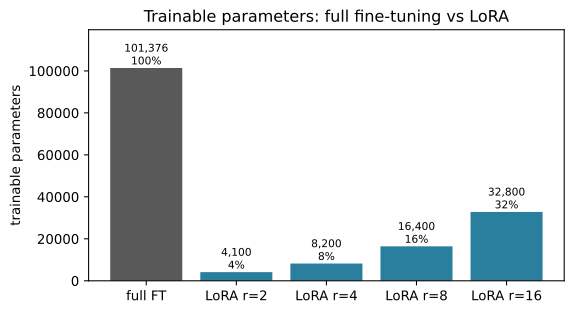
For contrast, we full-fine-tune the same task. A full update also reaches flip — and also forgets — but it moves all 101K parameters and produces a whole new checkpoint to store and serve, where the adapter is a few kilobytes bolted onto the shared base.
full_flip = copy.deepcopy(base)
fit(full_flip, make_stream("F", 800, seed=20), steps=300, lr=1.2e-3, seed=2)
print("full-FT flip:", round(accuracy(full_flip, "F"), 2),
      " echo kept:", round(accuracy(full_flip, "E"), 2))
full-FT flip: 1.0 echo kept: 0.0QLoRA attacks the other cost: holding the frozen base in memory during training (Dettmers et al. 2023). It stores the base weights in four-bit NormalFloat (NF4), a sixteen-value codebook whose points are spaced by the quantiles of a normal distribution — dense near zero, sparse in the tails, with an exact zero. It dequantizes to compute and backpropagates through that fixed reconstruction into the adapter. Figure 11.3 shows why the codepoints cluster where weights actually live.
# @save
NF4 = torch.tensor(
    [-1.0, -0.6961928, -0.5250731, -0.3949175, -0.2844414, -0.1847734,
     -0.0910500, 0.0, 0.0795803, 0.1609302, 0.2461123, 0.3379152,
     0.4407098, 0.5626170, 0.7229568, 1.0]
)


def nf4_quantize(weight: Tensor, group_size: int = 32) -> Tensor:
    """Round a weight tensor to the NF4 codebook, per absmax-scaled group.

    Each contiguous group of ``group_size`` values is divided by its largest
    magnitude, snapped to the nearest of the sixteen NF4 code points, and
    rescaled. Smaller groups track local scale better at the cost of more
    stored scales — the quantization-granularity trade-off of @sec-ch10.

    Args:
        weight: The full-precision weight tensor to quantize.
        group_size: Number of consecutive values sharing one absmax scale.

    Returns:
        The dequantized reconstruction, the same shape as ``weight``.
    """
    flat = weight.flatten()
    restored = torch.empty_like(flat)
    for s in range(0, flat.numel(), group_size):
        group = flat[s:s + group_size]
        scale = group.abs().max().clamp_min(1e-12)
        codes = (group / scale).unsqueeze(1).sub(NF4).abs().argmin(1)
        restored[s:s + group_size] = NF4[codes] * scale
    return restored.view_as(weight)
Show the code that draws this figure
import numpy as np
import matplotlib.pyplot as plt

xs = np.linspace(-3, 3, 400)
fig, ax = plt.subplots(figsize=(6.6, 3.2))
ax.plot(xs, np.exp(-xs ** 2 / 2) / np.sqrt(2 * np.pi), color="0.5")
ax.vlines(NF4.numpy() * 3, 0, 0.16, color="#b7791f", label="NF4 code points")
ax.vlines(np.linspace(-1, 1, 16) * 3, 0.17, 0.22, color="0.7", label="uniform 4-bit")
ax.set_xlabel("weight value (scaled to a standard normal)")
ax.set_yticks([])
ax.legend(loc="upper right", fontsize=8)
ax.set_title("NF4 spends its 16 levels where weights actually are")
plt.show()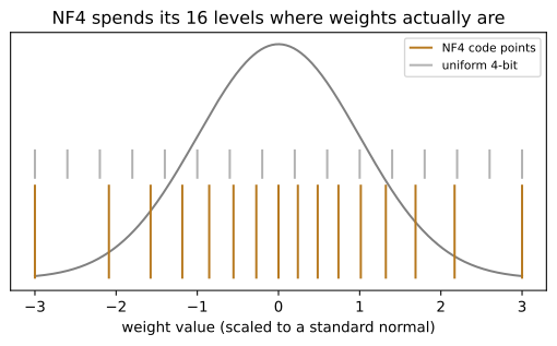
We quantize the base’s targeted matrices, confirm the frozen four-bit model still holds its capabilities, then train a LoRA adapter on top of it. Figure 11.4 traces which representation stores, which computes, and which updates.
qbase = copy.deepcopy(base)
squared_error = total = 0
with torch.no_grad():
    for block in qbase.blocks:
        for sub in ("attention", "mlp"):
            for name, m in getattr(block, sub).named_children():
                if name in TARGETS and isinstance(m, nn.Linear):
                    q = nf4_quantize(m.weight.data)
                    squared_error += ((q - m.weight.data) ** 2).sum().item()
                    total += m.weight.numel()
                    m.weight.data = q
print(f"NF4 reconstruction RMSE: {(squared_error / total) ** 0.5:.4f}")
print("quantized base still:", {op: round(accuracy(qbase, op), 2) for op in "EA"})

torch.manual_seed(2)
qlora = attach_lora(qbase, rank=4, alpha=8)
lora_parameters(qlora)
fit(qlora, make_stream("F", 800, seed=20), steps=300, lr=4e-3, seed=2)
print("QLoRA flip accuracy:", round(accuracy(qlora, "F"), 2))
NF4 reconstruction RMSE: 0.0038
quantized base still: {'E': 1.0, 'A': 1.0}
QLoRA flip accuracy: 1.0flowchart LR
X(["activation x"]) --> Q["frozen NF4 codes + scales"]
Q -->|"dequantize"| W["base matmul in higher precision"]
X --> A["trainable A"]
A --> Bm["trainable B"]
W --> SUM(("+"))
Bm -->|"scaled low-rank update"| SUM
SUM --> H(["activation h"])
L["loss"] -.->|"gradient"| Bm
L -.->|"gradient"| A
L -.->|"no update"| Q
The four-bit base reconstructs the weights to about four thousandths RMSE and keeps both capabilities intact, and the adapter reaches the same flip accuracy as the full-precision LoRA. The lesson is the QLoRA bargain: pay a small reconstruction error on the frozen base to cut its memory, and let the higher-precision adapter carry the learning. Rank-stabilized LoRA (scaling by \alpha/\sqrt{r}) and DoRA (separating weight magnitude from direction) are variants to evaluate under the same gate; neither repairs bad supervision.
11.3 Distillation moves behavior into a smaller model
Our flip model works, but it is the full 100K-parameter base. Suppose serving cost forces something smaller. Distillation trains a small student to reproduce a larger teacher on a declared operating distribution. It does not copy an abstract capability; what transfers depends on the prompts, the targets, and the loss. We take the full-fine-tuned flip model as the teacher and a student four times smaller.
teacher = full_flip  # a d=64 flip specialist, 101K parameters
def new_student():
    torch.manual_seed(7)
    return small_gpt(d_model=32, n_layers=2, n_heads=2)
print("teacher params:", sum(p.numel() for p in teacher.parameters()),
      " student params:", sum(p.numel() for p in new_student().parameters()))
teacher params: 101376 student params: 26016Sequence-level distillation samples the teacher’s completions and uses them as ordinary SFT targets. It works through a black-box API and can transfer format, tone, or solution traces, but it keeps only the teacher’s single chosen token and inherits its sampling errors. Logit distillation uses the teacher’s whole distribution. That distribution is where the teaching is: for one flip prompt, the teacher is almost sure of the right digit but places its small residual mass on the near-miss digits — the “dark knowledge” a hard label throws away.
@torch.no_grad()
def teacher_distribution(model, op, seed):
    rng = np.random.default_rng(seed)
    p = list(rng.integers(0, 10, size=NDIG))
    prompt = op + "".join(map(str, p)) + "="
    logits, _, _ = model(torch.tensor([[STOI[c] for c in prompt]]))
    return prompt, OPS[op](p)[0], logits[0, -1].softmax(-1)

prompt, truth, probs = teacher_distribution(teacher, "F", seed=3)
top = probs.topk(4)
print(f"prompt {prompt}  correct first answer digit: {truth}")
for value, index in zip(top.values.tolist(), top.indices.tolist()):
    print(f"  {ALPHABET[index]!r}: {value:.3f}")
prompt F8012= correct first answer digit: 1
'1': 0.993
'7': 0.002
'2': 0.001
'4': 0.001Logit distillation matches the softened teacher and student distributions. Let z_T, z_S be teacher and student logits and \tau > 0 a temperature; the objective contains
\mathcal{L}_{KD} = \tau^{2}\, D_{KL}\!\big(\operatorname{softmax}(z_T/\tau)\,\big\|\,\operatorname{softmax}(z_S/\tau)\big). \tag{11.2}
Temperature spreads the probability mass so the relative sizes of the wrong answers become a real training signal; the \tau^{2} factor compensates for the gradient shrinkage \tau introduces. Figure 11.5 shows one teacher distribution softening as \tau rises.
Show the code that draws this figure
import matplotlib.pyplot as plt

_, _, raw = teacher_distribution(teacher, "F", seed=3)
logit_vec = raw.clamp_min(1e-9).log()
digits = list(range(10))
fig, ax = plt.subplots(figsize=(6.6, 3.2))
for tau, color in [(1.0, "0.2"), (2.0, "#2a7f9e"), (4.0, "#b7791f")]:
    soft = (logit_vec[:10] / tau).softmax(0)
    ax.plot(digits, soft.numpy(), marker="o", ms=4, color=color, label=f"tau={tau:g}")
ax.set_xlabel("answer digit")
ax.set_ylabel("teacher probability")
ax.set_xticks(digits)
ax.legend()
ax.set_title("Temperature exposes the teacher's dark knowledge")
plt.show()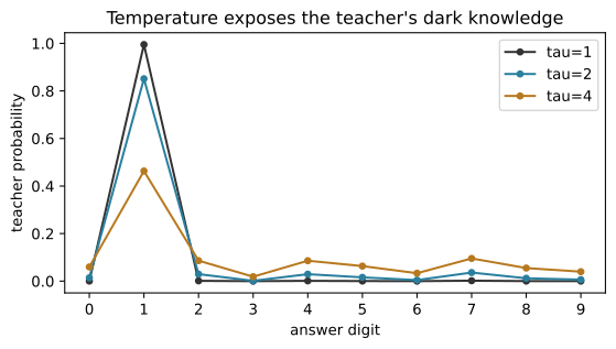
Now the executed comparison. We give a small student only 40 labeled examples and train it three ways: on the ground-truth labels (hard SFT), on the teacher’s greedy completions (sequence KD), and on the teacher’s softened answer-position distributions (logit KD). Distilling only the answer positions matters — the teacher has nothing useful to say about the random prompt digits.
# @save
def answer_positions(x: Tensor) -> Tensor:
    """Mark the ``NDIG`` positions after each ``=`` — where the answer is written.

    Distillation targets these positions only; the prompt digits are random and
    carry no transferable signal.

    Args:
        x: A batch of token id windows.

    Returns:
        A boolean mask, True on answer-token positions.
    """
    mask = torch.zeros_like(x, dtype=torch.bool)
    for b in range(x.size(0)):
        row = x[b].tolist()
        for t in range(x.size(1)):
            if row[t] == EQ:
                for k in range(NDIG):
                    if t + k < x.size(1):
                        mask[b, t + k] = True
    return mask


@torch.no_grad()
def teacher_completions(teacher, op, n, seed):
    """Build a training stream from the teacher's own greedy answers.

    This is sequence-level distillation: the student will imitate whatever the
    teacher writes, right or wrong, with no access to its distribution.

    Args:
        teacher: The model whose completions become labels.
        op: The operation tag to prompt with.
        n: Number of prompts to generate answers for.
        seed: Seed for the prompts.

    Returns:
        A token stream of ``op<digits>=<teacher answer>|`` examples.
    """
    rng = np.random.default_rng(seed)
    teacher.eval()
    parts = []
    for _ in range(n):
        p = list(rng.integers(0, 10, size=NDIG))
        prompt = op + "".join(map(str, p)) + "="
        out = generate(teacher, torch.tensor([[STOI[c] for c in prompt]]), NDIG, temperature=0.0)
        parts.append("".join(ALPHABET[i] for i in out[0].tolist()) + "|")
    return torch.tensor([STOI[c] for c in "".join(parts)], dtype=torch.long)


def distill_logits(student, teacher, stream, steps, lr, tau=2.0, alpha=0.7, size=64, seed=7, warmup=20):
    """Train a student on the teacher's softened answer distribution plus labels.

    The loss blends the temperature-scaled KL of @eq-ch11-kd (weight ``alpha``)
    with the ordinary hard-label cross-entropy, both restricted to answer
    positions. The ``tau**2`` factor keeps the soft term's gradient scale
    comparable to the hard term's.

    Args:
        student: The model being trained.
        teacher: The frozen teacher providing target logits.
        stream: The (small) training stream of real examples.
        steps: Number of optimizer steps.
        lr: Peak learning rate.
        tau: Softmax temperature applied to both models.
        alpha: Weight on the soft KL term versus the hard term.
        size: Batch size.
        seed: Seed for the window sampler.
        warmup: Linear-warmup steps.

    Returns:
        The list of per-step blended losses.
    """
    opt = torch.optim.AdamW(student.parameters(), lr=lr)
    gen = torch.Generator().manual_seed(seed)
    teacher.eval()
    losses = []
    for step in range(steps):
        for group in opt.param_groups:
            group["lr"] = lr * min(1.0, (step + 1) / warmup)
        x, y = batch(stream, size, gen)
        with torch.no_grad():
            t_logits, _, _ = teacher(x)
        s_logits, _, _ = student(x)
        m = answer_positions(x)
        p_t = (t_logits[m] / tau).softmax(-1)
        logp_s = (s_logits[m] / tau).log_softmax(-1)
        soft = -(p_t * logp_s).sum(-1).mean() * tau * tau
        hard = F.cross_entropy(s_logits[m], y[m])
        loss = alpha * soft + (1 - alpha) * hard
        opt.zero_grad(set_to_none=True)
        loss.backward()
        torch.nn.utils.clip_grad_norm_(student.parameters(), 1.0)
        opt.step()
        losses.append(loss.item())
    return losses
budget = 40
data = make_stream("F", budget, seed=31)
s_hard = new_student()
fit(s_hard, data, steps=400, lr=1.5e-3, seed=7)
s_seq = new_student()
fit(s_seq, teacher_completions(teacher, "F", budget, seed=31), steps=400, lr=1.5e-3, seed=7)
s_logit = new_student()
distill_logits(s_logit, teacher, data, steps=400, lr=1.5e-3)
distilled = {"teacher": accuracy(teacher, "F"), "hard SFT": accuracy(s_hard, "F"),
"sequence KD": accuracy(s_seq, "F"), "logit KD": accuracy(s_logit, "F")}
print({k: round(v, 2) for k, v in distilled.items()}){'teacher': 1.0, 'hard SFT': 0.26, 'sequence KD': 0.26, 'logit KD': 0.99}The gap is the point. With forty examples the student learns almost nothing from hard labels, and sequence KD is no better — with an accurate teacher its completions are the same forty hard targets. Logit KD, handed the teacher’s full distribution over each answer, nearly matches the teacher. Figure 11.6 shows all four.
Show the code that draws this figure
import matplotlib.pyplot as plt

names = list(distilled)
vals = [distilled[k] for k in names]
fig, ax = plt.subplots(figsize=(6.4, 3.4))
colors = ["0.35", "#c05a5a", "#c99a3a", "#2a7f9e"]
bars = ax.bar(names, vals, color=colors)
for bar, v in zip(bars, vals):
    ax.text(bar.get_x() + bar.get_width() / 2, v + 0.02, f"{v:.2f}", ha="center", fontsize=9)
ax.set_ylabel("flip accuracy (per character)")
ax.set_ylim(0, 1.1)
ax.set_title(f"Distilling flip into a 4x-smaller student ({budget} examples)")
plt.show()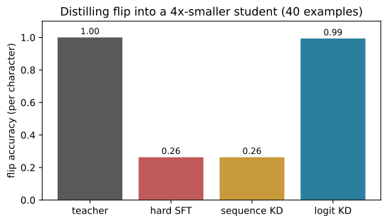
Two caveats keep this honest. The direction of the KL matters: forward KL, D_{KL}(p_T \| p_S), penalizes a student that fails to cover the teacher’s mass; reverse KL emphasizes the modes the student already commits to, which the MiniLLM work argues suits generative students (Gu et al. 2023). And static teacher completions train the student on teacher prefixes, while deployment feeds it its own prior tokens — the exposure mismatch that on-policy distillation addresses by letting the student generate and asking the teacher to grade those states (Agarwal et al. 2023). Reasoning traces add a further constraint we take on faith here rather than execute: a correct but very long teacher solution can exceed a small student’s capacity, and evidence on the learnability gap finds that sub-3-billion-parameter students often do better on shorter or mixed-length traces than on a strong teacher’s longest ones (Li et al. 2025). Treat trace length and abstraction as data-selection knobs, and use only outputs the license permits.
11.4 Merging combines task vectors, not capabilities
Two teams fine-tune the same base — one for flip, one for a second operation, shift — and want one model that does both without a joint retraining run. Merging tries to get it by arithmetic on the weights. For base parameters \theta_0 and a fine-tuned \theta_i, the task vector is \tau_i = \theta_i - \theta_0 (Ilharco et al. 2022), and linear merging forms \theta_0 + \sum_i \lambda_i \tau_i. LoRA makes this cheap: the task vector is already the realized delta (\alpha/r) B A. We first build the shift specialist.
torch.manual_seed(3)
lora_shift = attach_lora(copy.deepcopy(base), rank=4, alpha=8)
lora_parameters(lora_shift)
fit(lora_shift, make_stream("S", 800, seed=25), steps=300, lr=4e-3, seed=3)
print("shift adapter:", round(accuracy(lora_shift, "S"), 2))
shift adapter: 0.99We collect each adapter’s per-layer deltas and merge them two ways: plain weighted averaging, and TIES, which trims each delta to its largest-magnitude coordinates, elects a sign per coordinate, and averages only the sign-agreeing survivors — an attempt to keep the two updates from cancelling (Yadav et al. 2023).
# @save
def collect_deltas(model) -> dict:
    """Collect every LoRA layer's realized dense update as a task vector.

    Args:
        model: A model carrying ``LoRALinear`` adapters.

    Returns:
        A dict from ``(block_index, sublayer, name)`` to the dense delta
        ``(alpha/r)·B·A`` for that layer — the per-layer task vector to merge.
    """
    out = {}
    for i, block in enumerate(model.blocks):
        for sub in ("attention", "mlp"):
            for name, mod in getattr(block, sub).named_children():
                if isinstance(mod, LoRALinear):
                    out[(i, sub, name)] = mod.delta.detach()
    return out


def ties_merge(delta_a: Tensor, delta_b: Tensor, wa: float, wb: float, density: float = 0.6) -> Tensor:
    """Merge two weighted deltas by trim, sign-elect, and disjoint average.

    Each delta keeps only its top ``density`` fraction by magnitude; a sign is
    elected per coordinate from the weighted sum; only the survivors whose sign
    matches the elected sign are averaged. Opposed updates that would cancel in
    a plain average are dropped instead.

    Args:
        delta_a: The first task's dense update.
        delta_b: The second task's dense update.
        wa: Weight on the first update.
        wb: Weight on the second update.
        density: Fraction of each delta's coordinates to keep after trimming.

    Returns:
        The merged dense update, the shape of one input delta.
    """
    trimmed = []
    for d, w in ((delta_a, wa), (delta_b, wb)):
        k = max(1, int((1 - density) * d.numel()))
        cutoff = d.abs().flatten().kthvalue(k).values
        trimmed.append(torch.where(d.abs() >= cutoff, w * d, torch.zeros_like(d)))
    stack = torch.stack(trimmed)
    elected = torch.sign(stack.sum(0))
    keep = (torch.sign(stack) == elected).float()
    count = keep.sum(0).clamp_min(1)
    return (stack * keep).sum(0) / count


def merged_model(base_model, deltas_a, deltas_b, wa, wb, method):
    """Add a linear or TIES combination of two task vectors onto a base copy.

    Args:
        base_model: The shared base to merge onto.
        deltas_a: The first adapter's per-layer deltas from ``collect_deltas``.
        deltas_b: The second adapter's per-layer deltas.
        wa: Weight on the first task vector.
        wb: Weight on the second task vector.
        method: ``"linear"`` for weighted sum, ``"ties"`` for the TIES rule.

    Returns:
        A new model whose targeted weights carry the merged update.
    """
    m = copy.deepcopy(base_model)
    with torch.no_grad():
        for i, block in enumerate(m.blocks):
            for sub in ("attention", "mlp"):
                for name, mod in getattr(block, sub).named_children():
                    key = (i, sub, name)
                    if key in deltas_a:
                        d = (ties_merge(deltas_a[key], deltas_b[key], wa, wb)
                             if method == "ties" else wa * deltas_a[key] + wb * deltas_b[key])
                        mod.weight.data = mod.weight.data + d
    return m
We sweep the flip/shift blend from all-shift to all-flip, scoring both tasks at every point.
deltas_flip, deltas_shift = collect_deltas(lora_flip), collect_deltas(lora_shift)
sweep = []
for wa in (0.0, 0.2, 0.4, 0.5, 0.6, 0.8, 1.0):
    for method in ("linear", "ties"):
        mm = merged_model(base, deltas_flip, deltas_shift, wa, 1 - wa, method)
        fa, sa = accuracy(mm, "F", n=100), accuracy(mm, "S", n=100)
        sweep.append((method, wa, fa, sa, (fa + sa) / 2))
eq = {m_: (f, s, mean) for (m_, w, f, s, mean) in sweep if w == 0.5}
print("50/50 merge  linear:", {k: round(v, 2) for k, v in zip("F S mean".split(), eq["linear"])})
print("50/50 merge  ties:  ", {k: round(v, 2) for k, v in zip("F S mean".split(), eq["ties"])})
50/50 merge linear: {'F': 0.43, 'S': 0.25, 'mean': 0.34}
50/50 merge ties: {'F': 0.17, 'S': 0.36, 'mean': 0.27}The 50/50 model does each task only partially — around 0.5 on flip and 0.35 on shift with linear merging, worse still with TIES. Figure 11.7 draws the whole sweep, and its shape is the honest lesson: as we shift weight from shift to flip, flip accuracy rises while shift accuracy falls, and the mean dips in the middle. The two task vectors interfere; a blend is worse at each task than the corresponding specialist, and neither linear nor TIES conjures a model that is good at both. Merging combines updates, not capabilities.
Show the code that draws this figure
import matplotlib.pyplot as plt

fig, ax = plt.subplots(figsize=(6.6, 3.6))
lin = [r for r in sweep if r[0] == "linear"]
was = [r[1] for r in lin]
ax.plot(was, [r[2] for r in lin], marker="o", color="#2a7f9e", label="flip accuracy")
ax.plot(was, [r[3] for r in lin], marker="s", color="#b7791f", label="shift accuracy")
ax.plot(was, [r[4] for r in lin], ls="--", color="0.4", label="mean (linear)")
ax.plot(was, [r[4] for r in sweep if r[0] == "ties"], ls=":", color="0.4", label="mean (TIES)")
ax.set_xlabel("weight on the flip task vector")
ax.set_ylabel("accuracy")
ax.set_ylim(0, 1.05)
ax.legend(fontsize=8)
ax.set_title("A two-task merge trades one capability for the other")
plt.show()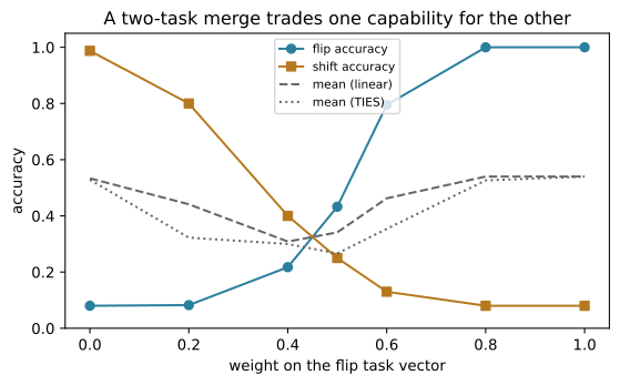
Merging earns its place when training data are unavailable, when ablation is cheap, or when one artifact simplifies serving — and when the tasks are compatible enough that the blend holds up. When they conflict, as here, the better answer is to keep the adapters separate and route between them, which is exactly what multi-adapter serving does (Section 11.7). Merging requires aligned parameters — same architecture, tokenizer, and normally the same base revision — and it inherits every source model’s license and risk; matching filenames is not enough.
11.5 Catastrophic forgetting and the four-set gate
We already saw the flip adapter erase echo and add-one. A frozen base does not guarantee preserved behavior, because inference runs W_0 + \Delta W, and the update can dominate an activation: for any input, \lVert (\alpha/r) B A x\rVert \le (\alpha/r)\lVert B\rVert\,\lVert A\rVert\,\lVert x\rVert, a bound that grows with rank and scale. Catastrophic forgetting is measured behavior on old capabilities, not proof that base tensors moved. We demonstrate it head-on: fine-tune the generalist hard on shift, then measure echo and add-one.
NoteIn the interview
Q — If LoRA freezes the base weights, how can training an adapter degrade the model’s other capabilities? Because inference uses W_0 + \Delta W, not W_0. The adapter adds a term to every targeted activation, and Equation 11.1 shows that term can be large relative to the base output — a frozen matrix is not frozen behavior. The trap is treating “base weights unchanged” as “old behavior safe” and shipping without a regression set. Always measure the capabilities you care about after tuning, on data the adapter never saw.
forget_stages = {}
forget_stages["base"] = {op: accuracy(base, op) for op in "EAS"}

ft_shift = copy.deepcopy(base)
fit(ft_shift, make_stream("S", 800, seed=25), steps=350, lr=1.2e-3, seed=2)
forget_stages["fine-tuned on shift"] = {op: accuracy(ft_shift, op) for op in "EAS"}
print("after fine-tuning on shift:", {op: round(v, 2) for op, v in forget_stages["fine-tuned on shift"].items()})
after fine-tuning on shift: {'E': 0.2, 'A': 0.27, 'S': 1.0}Shift went from chance to solved, and echo and add-one collapsed with it. The standard repair is replay: mix a representative slice of the old capabilities back into the training data so the gradient keeps seeing them.
replay = copy.deepcopy(base)
fit(replay, make_stream(["S", "E", "A"], 900, seed=26), steps=350, lr=1.2e-3, seed=2)
forget_stages["replay mix"] = {op: accuracy(replay, op) for op in "EAS"}
print("after replay mix:", {op: round(v, 2) for op, v in forget_stages["replay mix"].items()})
after replay mix: {'E': 1.0, 'A': 1.0, 'S': 0.98}The replay-trained model learns shift and keeps echo and add-one — one model, all three, no forgetting. Figure 11.8 tells the story in three bars.
Show the code that draws this figure
import matplotlib.pyplot as plt
import numpy as np

stages = list(forget_stages)
ops = ["E", "A", "S"]
labels = {"E": "echo (old)", "A": "add-one (old)", "S": "shift (new)"}
x = np.arange(len(stages))
width = 0.26
fig, ax = plt.subplots(figsize=(6.8, 3.6))
for j, op in enumerate(ops):
    ax.bar(x + (j - 1) * width, [forget_stages[s][op] for s in stages], width, label=labels[op])
ax.set_xticks(x)
ax.set_xticklabels(stages)
ax.set_ylabel("accuracy")
ax.set_ylim(0, 1.1)
ax.legend(fontsize=8)
ax.set_title("Forgetting, and the replay mix that repairs it")
plt.show()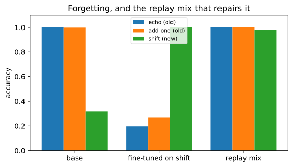
Measuring this needs discipline about which data does what. A customization project needs four data roles with different access rules — the four-set design:
| Set | Used for | Never used for | Failure it catches |
|---|---|---|---|
| Train | gradient updates | reporting generalization | memorization, imbalance |
| Development | recipe, checkpoint, mixture choice | the final claim | overfitting to train |
| Task test | one release decision, recipe frozen | iterative tuning | true in-scope generalization |
| Regression | old capability, safety, cost | optimizing an aggregate | collateral damage |
The task test is untouched by construction — decontaminate it by source, template, and semantic overlap, and rotate it once it has been inspected too often. Then predeclare a ship rule. Let \Delta M be the task-test gain, \Delta R_j each regression drop, \delta the required gain, and \epsilon_j each tolerated loss:
\operatorname{ship} = \mathbf{1}\big[\Delta M \ge \delta \ \wedge\ \forall j:\ \Delta R_j \le \epsilon_j\big]. \tag{11.3}
Our regression set is the old echo and add-one behaviors; the gate refuses any candidate that buys shift by wrecking them.
# @save
def release_gate(baseline, candidate, task_op, regression_ops, min_gain=0.30, max_drop=0.05):
    """Decide whether a candidate ships, given a task gain and regression budget.

    Implements @eq-ch11-gate: the candidate must improve the task set by at
    least ``min_gain`` and must not drop any regression capability by more than
    ``max_drop``. A large task gain cannot buy an unacceptable regression.

    Args:
        baseline: ``{op: accuracy}`` for the pre-tuning model.
        candidate: ``{op: accuracy}`` for the tuned model.
        task_op: The operation whose gain is required.
        regression_ops: Operations that must be preserved.
        min_gain: Minimum required task-set gain.
        max_drop: Maximum tolerated drop on any regression op.

    Returns:
        A dict with the measured gain, the worst drop, and the ship decision.
    """
    gain = candidate[task_op] - baseline[task_op]
    worst_drop = max(baseline[o] - candidate[o] for o in regression_ops)
    return {"gain": round(gain, 3), "worst_regression_drop": round(worst_drop, 3),
            "ship": bool(gain >= min_gain and worst_drop <= max_drop)}
base_scores = forget_stages["base"]
print("fine-tuned-on-shift candidate:",
release_gate(base_scores, forget_stages["fine-tuned on shift"], "S", "EA"))
print("replay candidate: ",
release_gate(base_scores, forget_stages["replay mix"], "S", "EA"))fine-tuned-on-shift candidate: {'gain': 0.68, 'worst_regression_drop': 0.803, 'ship': False}
replay candidate: {'gain': 0.662, 'worst_regression_drop': 0.0, 'ship': True}Both candidates clear the task-gain bar by a wide margin; only the replay candidate clears the regression bar, so only it ships. The gate is the mechanism that turned “the model got better at shift” into a defensible release decision — and it is where data engineering pays off. Figure 11.9 places the irreversible boundary at dataset approval and keeps the test and regression sets outside any self-improvement loop.
flowchart LR
    P["versioned real prompts + labels"] --> SPL["split by source / entity"]
    SPL --> TR["train"]
    SPL --> DV["development"]
    SPL --> TT["sealed task test"]
    SPL --> RG["regression suite"]
    TR --> GEN["teacher / policy generates candidates"]
    GEN --> FLT["executable checks, dedup, license filter"]
    FLT -->|"approved + provenance"| MIX["versioned training mixture"]
    MIX --> TRN["SFT / preference / RFT / distill"]
    TRN --> GEN
    DV -->|"recipe only"| MIX
    TRN --> CAND["release candidate"]
    TT --> CAND
    RG --> CAND
Synthetic data is a measurement instrument, not free truth: Self-Instruct bootstraps instructions from a model and filters them (Wang et al. 2023), rejection sampling keeps only verifier-passing outputs, and each loop can narrow diversity or amplify a grader’s blind spot. Split by source before you synthesize, keep licensed human or executable anchors, and stop when held-out improvement saturates.
11.6 Preference tuning, reinforcement fine-tuning, and pruning
SFT treats every target token as equally authoritative. When several responses are valid but one is preferred — less hedging, a cleaner refusal, the right tone — comparative feedback fits better. Preference tuning collects a chosen and a rejected response to the same prompt and optimizes the margin between them relative to a reference policy. Chapter 7 derives the DPO loss; the shape is a logistic on the reference-relative margin, and the point here is only that it is a small, surgical intervention.
import math

def dpo_margin_loss(chosen, rejected, ref_chosen, ref_rejected, beta=0.1):
    margin = beta * ((chosen - ref_chosen) - (rejected - ref_rejected))
    return -math.log(1 / (1 + math.exp(-margin)))

# same reference; policy prefers the chosen response vs prefers the rejected one
print("aligned  :", round(dpo_margin_loss(-2.0, -3.0, -2.5, -2.5), 3))
print("misaligned:", round(dpo_margin_loss(-3.0, -2.0, -2.5, -2.5), 3))
aligned : 0.644
misaligned: 0.744The loss is low when the policy raises the chosen response’s log-probability above the rejected one relative to the reference, and high when it does the reverse — a tone or refusal fix, not a way to inject a quarterly policy document. Reinforcement fine-tuning goes further when a reliable scalar verifier exists — tests that pass, a checked final answer, a validator — and Chapter 8 owns its mechanics (Chapter 23 extends it to full agent trajectories). Its first failure mode is the grader: if formatting or leaked references can raise reward without solving the task, the model will find that path, so evaluate the grader on held-out good and bad outputs before trusting it.
Compression creates a smaller model rather than an adapter. Structured pruning removes whole heads, channels, or layers and needs recovery training; the Minitron line prunes then distills to recover quality (Muralidharan et al. 2024), and SliceGPT deletes rows and columns after rotations that preserve the network’s function (Ashkboos et al. 2024). Low-rank compression factorizes an existing matrix W \in \mathbb{R}^{m\times n} as a rank-k product, cutting parameters from mn to k(m+n). A truncated SVD minimizes reconstruction error — which is not the same as minimizing language-model loss, the caveat worth executing on one of our own weight matrices.
W = teacher.blocks[0].mlp.down.weight.detach()
U, S, Vt = torch.linalg.svd(W, full_matrices=False)
for k in (2, 8, 16):
    approx = (U[:, :k] * S[:k]) @ Vt[:k]
    rel_err = (W - approx).norm() / W.norm()
    print(f"rank {k:2d}: {k * (W.shape[0] + W.shape[1]):5d} params "
          f"(vs {W.numel()}), reconstruction error {rel_err:.2f}")
rank 2: 470 params (vs 10944), reconstruction error 0.87
rank 8: 1880 params (vs 10944), reconstruction error 0.61
rank 16: 3760 params (vs 10944), reconstruction error 0.43Even keeping rank 16 of this matrix leaves a large reconstruction error; how much of that becomes lost accuracy is an empirical question the gate has to answer, because Frobenius error and task loss are different objectives. Quantization is another compression axis, but Chapter 10’s validation ladder stays authoritative, and each composition of pruning, distillation, and quantization needs its own measurement.
11.7 Serving customized models
Training produces an artifact; serving gives it identity, latency, and a blast radius. Register the whole lineage — base and tokenizer revisions, chat template, quantization recipe, adapter or merged weights, data manifest, evaluation record, and approval — because a hash of the adapter file alone cannot detect a mismatched base.
The unmerged-versus-merged choice is a real trade. An unmerged adapter keeps a tiny artifact, instant rollback, and multi-tenant sharing — many adapters over one base, the multi-LoRA serving path Chapter 10 owns — at the cost of adapter loading and routing in the serving lattice. A merged checkpoint simplifies the runtime and removes adapter lookup, but consumes a full artifact, weakens revocability, and demands another quantization and regression pass. When two task vectors conflict, as flip and shift did, separate adapters are also simply better than a merge.
QLoRA makes merging numerically delicate. The training base is a four-bit reconstruction while a higher-precision checkpoint may also exist; adding \Delta W to one and serving the other changes the model, and repeatedly merging into four-bit codes re-quantizes the sum. Choose the target representation explicitly: dequantize the intended base, merge in adequate precision, quantize once under a pinned recipe, then rerun the gate. The real seven-billion-parameter path is the same mechanism at scale — an NF4 base, a rank-16 adapter, all-linear targets — which we show as configuration, not as a run:
# Representative real-scale QLoRA seam (illustrative config, not executed here).
from transformers import AutoModelForCausalLM, BitsAndBytesConfig
from peft import LoraConfig, get_peft_model

quant = BitsAndBytesConfig(load_in_4bit=True, bnb_4bit_quant_type="nf4",
                           bnb_4bit_use_double_quant=True, bnb_4bit_compute_dtype="bfloat16")
model = AutoModelForCausalLM.from_pretrained("<open-weight-base>", quantization_config=quant)
model = get_peft_model(model, LoraConfig(
    r=16, lora_alpha=32, lora_dropout=0.05, task_type="CAUSAL_LM",
    target_modules=["q_proj", "k_proj", "v_proj", "o_proj", "gate_proj", "up_proj", "down_proj"]))
model.print_trainable_parameters()  # the same tiny fraction we counted above
The defaults above pin the mechanism, not an optimum — sweep rank, learning rate, epochs, and data mixture on development data, and score all four sets before shipping. Then canary on the traffic slice the test set represents, with a base-model fallback and an adapter kill switch, and admit production corrections as training data only through the governed boundary of Figure 11.9.
Verified on 2026-07-19. The open-weight stack exposes this chapter as libraries. Hugging Face PEFT documents LoRA, rsLoRA, DoRA, quantized-training preparation, and adapter merging; bitsandbytes documents NF4, double quantization, and the compute dtype; TRL provides SFT and DPO trainers; mergekit implements task-arithmetic, TIES, DARE, and SLERP merges. Managed customization now spans SFT, preference tuning, and grader-driven RFT across major providers, each restricting available bases, exportability, and data retention differently. Hosted tuning buys managed training and deployment but limits gradients, logits, merging, and export; open-weight DIY grants tensor-level control while making you responsible for kernels, licenses, and serving. Choose from the control surface you need, not from ideology. Verify live: tunable model IDs and retirement dates; SFT/preference/RFT/distillation availability; logit and weight export rights; PEFT/bitsandbytes/serving-engine compatibility; adapter and merge support in your inference stack; prices, quotas, and licenses.
11.8 Summary
Customization starts by not customizing: diagnose whether the failure is evidence, state, effect, representation, behavior, or economics, and touch weights only for the last two. When you do, match the method to your supervision. LoRA trains a rank-bounded update — here 8% of the model — over a frozen base; QLoRA holds that base in four bits for nearly the same result. Distillation moves behavior into a smaller student, where the teacher’s full distribution beat its hard labels. Merging adds task vectors and pays for their interference; a frozen base still forgets, and a replay mix repairs it. Every path returns to a four-set gate. Chapter 14 completes the evidence branch.
11.9 Exercises
Refuse to train. Take a real failure and classify it against the six branches of Figure 11.1. Build the strongest prompt, schema, retrieval, and tool baseline the interface allows, run it on a frozen set, and state precisely what new evidence would justify SFT, preference tuning, or RFT — and why training before that evidence would be premature.
Budget a LoRA configuration. Using Equation 11.1, compute the trainable parameters for ranks 2, 8, 16, and 64 on the tinygpt, and re-run the flip fine-tune at each. Plot flip accuracy against rank and against \alpha. Where do returns stop, and does \alpha/\sqrt{r} scaling change the picture at high rank?
Make distillation earn its gap. Sweep the distillation budget (
budget) from 20 to 400 examples for all three students (hard, sequence, logit KD). At what data size does the logit-KD advantage vanish, and why? Then raise the temperaturetauindistill_logitsto 1, 2, and 4 and explain the effect on the small-data regime.Break and fix a merge. Add a third adapter for add-one and merge all three. (a) Find any weighting where the mean of the three tasks beats every pair of separate adapters, or argue from the sweep why none exists. (b) Sweep the TIES
densityfrom 0.2 to 0.9 and report where, if anywhere, TIES overtakes linear merging. (c) Decide whether routing three separate adapters is safer than any merge.Operate the four-set gate. Replace the point thresholds in
release_gatewith at least three regression slices and a paired confidence interval. Then simulate ten rounds of recipe selection that repeatedly peek at the “task test,” show how the ship decision drifts optimistic, and design a rotation policy that restores it.Quantify forgetting against the update norm. For the flip adapter, sweep rank and \alpha and, at each setting, record both flip accuracy and the echo/add-one regression alongside the operator-norm bound \lVert(\alpha/r)BA\rVert from Section 11.5. Do the regression drops track the bound? Find the smallest intervention that passes the gate.
Distill, then serve. Take the logit-KD student, quantize it under Chapter 10’s ladder, and compare it with the teacher and with a from-scratch model of the student’s size trained on the full data. Report accuracy, parameter count, and the break-even query volume at which distilling was worth its build cost, then write the model-card lineage you would ship.