# @save
from __future__ import annotations

from typing import Any

from opentelemetry.sdk.trace import TracerProvider
from opentelemetry.sdk.trace.export import SimpleSpanProcessor
from opentelemetry.sdk.trace.export.in_memory_span_exporter import InMemorySpanExporter
from opentelemetry.trace import Link


def build_tracer() -> tuple[Any, InMemorySpanExporter]:
    """Create an isolated in-memory OpenTelemetry pipeline for examples and tests.

    An in-memory exporter keeps the span tree in a Python list instead of
    shipping it to a collector, so the structure a run produces is something
    a test can read back and assert on. Production swaps this one object for
    an OTLP exporter and nothing else changes.

    Returns:
        The tracer to open spans with, and the exporter holding finished spans.
    """
    exporter = InMemorySpanExporter()
    provider = TracerProvider()
    provider.add_span_processor(SimpleSpanProcessor(exporter))
return provider.get_tracer("agentic-book-ch27"), exporter27 Operating Agents: Observability, SLOs, Incidents, and Privacy Ops
A support ticket says, “the agent got slow this week.” The API dashboard is green: 99.98 percent of requests return HTTP 200, median latency is flat, workers have spare CPU. A second chart reports 96.55 percent successful tasks and is also green, because its threshold is 95 percent. Both dashboards are telling the truth and both are missing the story. The service actually promised 99.5 percent successful, grounded journeys over 30 days, and a 96.55 percent result is burning that promise at almost seven times the rate it can afford — the budget for a whole month will be gone in about four days. “Slow” is one visible symptom of tool timeouts driving retries, retries driving cost, and some answers claiming success without the final state ever changing. An HTTP endpoint can be perfectly healthy while it hands a user an unauthorized refund, an unsupported answer, or a plan that loops until its currency budget expires.
We are now ready to build the small console that sees what those dashboards miss, and to build it the way we run it — in executed fragments whose numbers appear on the page. The parts are (i) a real OpenTelemetry span tree for one agent run, with a durable approval pause represented as two linked traces; (ii) four telemetry channels joined by stable identities, and a replay mode that repeats no effects; (iii) journey-level service-level indicators computed from a batch of runs; (iv) error-budget burn, days-to-exhaustion, and a multiwindow paging rule fired against a scripted bad deploy; (v) drift detection with its detection delay measured, and a canary decision from a two-proportion test; (vi) an error-budget policy that lowers autonomy, tested with one chaos drill; (vii) an incident run through both a technical and a business rollback, then frozen into a permanent regression test; (viii) human review operated as a queue we measure for discrimination and delay; and (ix) telemetry redaction that survives a false-positive we deliberately trip. Chapter 22 owns whether an offline evaluation supports a release; Chapter 26 owns gateways, durable effects, and delivery; this chapter owns runtime truth. The join key throughout is the journey identity from Chapter 26.
27.1 Trace one run without a three-day span
A trace is the causal record of one unit of work as it moves across components; a span is one bounded operation inside it, with a start, an end, a status, attributes, and a parent. Context propagation makes a client span the parent of a server span, so a whole request reads as a tree. That tree is exactly what the green HTTP dashboard cannot show: it aggregates over spans instead of preserving them. We build the smallest real version — the OpenTelemetry SDK writing to an in-memory exporter, so the structure is inspectable in a test with no collector running.
The hard case for tracing an agent is the durable pause. A run that requests human approval may wait minutes or days for a decision (the pause is Chapter 26’s durable-execution machinery). Holding one span open across that wait would report a three-day tool call and destroy every latency percentile. The fix is to end the trace when the computation suspends, persist the run and action identity, and start a new trace when the approval signal arrives — adding a link from the resumed root back to the first trace. A link says “related, but not a strict child,” which is exactly the relationship a resume has to its origin. Figure 27.1 shows the shape.
sequenceDiagram
    participant U as User
    participant A as Agent worker
    participant W as Durable workflow
    participant H as Review queue
    participant T as Effect tool
    U->>A: run-17
    rect rgb(238, 244, 250)
        Note over A: Trace 1
        A->>A: invoke_agent then chat
        A->>H: request_approval(action-17)
        A->>W: persist suspension + trace context
    end
    W-->>A: worker may stop
    H->>W: approved(action-17)
    rect rgb(238, 248, 242)
        Note over A: Trace 2, linked to Trace 1
        W->>A: resume_agent(run-17)
        A->>T: execute_tool(action-17)
        T-->>A: receipt-1
    end
Here is that run emitted for real. The first with block opens invoke_agent as a root, nests chat and request_approval under it, and captures the root’s span context before it closes. The second block opens resume_agent as a new root carrying a link to that captured context, and executes the tool beneath it.
# @save
def emit_linked_run() -> tuple[list[Any], str]:
    """Emit one agent run whose approval pause splits it into two linked traces.

    The first trace covers work up to the suspension and then ends, so the
    days spent waiting for a human never inflate a span. The second trace
    begins on resume and carries a ``Link`` to the first, which is how an
    observability backend reconstructs one journey from two bounded traces.

    Returns:
        The finished spans, and the first trace id as a hex string.
    """
    tracer, exporter = build_tracer()
    with tracer.start_as_current_span(
        "invoke_agent",
        attributes={"gen_ai.operation.name": "invoke_agent",
                    "app.run.id": "run-17", "app.release.hash": "bundle-42"},
    ) as first:
        with tracer.start_as_current_span(
            "chat",
            attributes={"gen_ai.operation.name": "chat",
                        "gen_ai.request.model": "fixture-model",
                        "gen_ai.usage.input_tokens": 20_000,
                        "gen_ai.usage.output_tokens": 2_000,
                        "app.cost": 0.013},
        ):
            pass
        with tracer.start_as_current_span(
            "request_approval", attributes={"app.action.id": "refund:A-17:v1"},
        ):
            pass
        first_context = first.get_span_context()
    with tracer.start_as_current_span(
        "resume_agent",
        links=[Link(first_context, attributes={"app.link.reason": "approval_resume"})],
        attributes={"app.run.id": "run-17", "app.approval.decision": "approve"},
    ):
        with tracer.start_as_current_span(
            "execute_tool",
            attributes={"gen_ai.operation.name": "execute_tool",
                        "app.action.id": "refund:A-17:v1",
                        "app.effect.receipt": "receipt-1"},
        ):
            pass
    return list(exporter.get_finished_spans()), f"{first_context.trace_id:032x}"
To see that the structure is what we claimed, we print the tree grouped by trace, chronological order, marking the link.
# @save
def print_span_tree(spans: list[Any]) -> None:
    """Print finished spans as one indented tree per trace, marking links.

    Grouping by trace and ordering by start time turns a flat span list back
    into the causal picture, and annotating the link shows how the resumed
    trace points home. This is the diagnostic view the aggregate dashboards
    threw away.

    Args:
        spans: Finished spans from an in-memory exporter.
    """
    by_trace: dict[int, list[Any]] = {}
    for span in spans:
        by_trace.setdefault(span.context.trace_id, []).append(span)
    ordered = sorted(by_trace.items(), key=lambda kv: min(s.start_time for s in kv[1]))
    number = {trace_id: i for i, (trace_id, _) in enumerate(ordered, start=1)}
    for trace_id, group in ordered:
        by_parent: dict[int | None, list[Any]] = {}
        for span in group:
            by_parent.setdefault(span.parent.span_id if span.parent else None, []).append(span)

        def walk(parent_id: int | None, depth: int) -> None:
            for span in sorted(by_parent.get(parent_id, []), key=lambda s: s.start_time):
                link = (f"   (links to trace {number[span.links[0].context.trace_id]})"
                        if span.links else "")
                print(f"trace {number[trace_id]}  " + "  " * depth + f"{span.name}{link}")
                walk(span.context.span_id, depth + 1)

        walk(None, 0)
spans, first_trace = emit_linked_run()
print_span_tree(spans)
print(f"\nspans={len(spans)} traces={len({s.context.trace_id for s in spans})} "
f"links={sum(len(s.links) for s in spans)}")trace 1 invoke_agent
trace 1 chat
trace 1 request_approval
trace 2 resume_agent (links to trace 1)
trace 2 execute_tool
spans=5 traces=2 links=1Five spans, two trace ids, one link — one journey, no absurd span. Moving from this in-memory exporter to a production backend is a one-object change; the instrumentation above is untouched.
from opentelemetry.exporter.otlp.proto.grpc.trace_exporter import OTLPSpanExporter

provider = TracerProvider()
provider.add_span_processor(SimpleSpanProcessor(
    OTLPSpanExporter(endpoint="http://localhost:4317")))
Two cautions travel with every trace. Name spans by operations a reader can reason about — invoke_agent, chat, execute_tool — and split attributes by namespace: gen_ai.* for the model operation, db.*/http.* for dependencies, and an app.* namespace for run, release, outcome, and cost fields. And never encode unbounded values — raw prompts, order ids, user ids — as metric labels; they blow up cardinality and copy personal data into an index, a hazard we disarm in Section 27.9. A trace is diagnostic evidence, not an immutable audit record: sampling, exporter loss, and retention are legitimate properties of a tracing system, which is why a span reporting status=success proves nothing about the world unless it carries a verifier-owned receipt.
27.2 Fan telemetry into four sources of truth
No single channel should answer billing, debugging, alerting, and audit at once; their reliability, volume, retention, and mutability needs conflict. A tracing outage must not erase the bill, and a sampled debugging store must not be asked to estimate the fleet failure rate. So a run fans out to four channels joined by the same stable identities, shown in Figure 27.2.
flowchart LR
    RUN["Agent journey<br/>run · attempt · release · tenant surrogate"] --> METRIC[("Unsampled metrics<br/>rates · latency · SLO")]
    RUN --> TRACE[("Sampled traces<br/>trajectory · timing")]
    RUN --> USAGE[("Unsampled usage ledger<br/>tokens · tools · cost")]
    RUN --> AUDIT[("Append-only effect audit<br/>policy · approval · receipt")]
    METRIC -. "exemplar / run id" .-> TRACE
    AUDIT -. "authoritative outcome" .-> METRIC
    USAGE -. "invoice reconciliation" .-> METRIC
The division of labor matters most where the channels seem to overlap. Metrics aggregate: a counter such as agent_journeys_total{release, outcome_class} is cheap and complete but cannot reconstruct one path. Traces are sampled, so a trace store deliberately over-retaining errors is superb for debugging and useless for estimating a rate. The usage ledger is unsampled and append-oriented because losing a span must not change the invoice — which is why cost read off traces can only ever be diagnostic. We make that word literal: the function that sums cost across spans is named for what it is.
# @save
def trace_cost(spans: list[Any]) -> float:
    """Sum the diagnostic cost carried on spans; the bill lives in the ledger.

    Reading cost from sampled traces is convenient for attributing spend to a
    trajectory during debugging, but a lost span would silently lower the
    total — so this number is a diagnostic estimate, never the amount a
    customer is charged.

    Args:
        spans: Finished spans that may carry an ``app.cost`` attribute.

    Returns:
        The summed cost, rounded, for diagnostic display only.
    """
    return round(sum(float(s.attributes.get("app.cost", 0.0)) for s in spans), 6)
The run’s spans carry one cost attribute, which we read as a diagnostic total.
print("diagnostic_trace_cost =", trace_cost(spans))diagnostic_trace_cost = 0.013The fourth channel, the append-only effect audit, records proposed and authorized actions, policy version, approval evidence, and provider receipts; its access is more restricted than ordinary traces because those records carry decision context. Immutability and independent anchoring of that audit belong to Chapter 24. One operational habit stitches the channels together: reconciliation jobs that detect missing joins — an effect receipt with no run, metered usage with no tenant, a completed journey with no authoritative outcome. The console can then distinguish evidence is absent from the event is absent, a difference a single dashboard blurs.
The channels also constrain how we debug. Replay is a diagnostic mode, not a second production execution: it reconstructs model inputs from retained content and re-runs deterministic code, but write tools must go through a no-effect adapter, or a replay of a refund becomes a new incident. The adapter is tiny and worth seeing, because its whole job is to make effects impossible.
# @save
def replay_execute(name: str, arguments: dict[str, Any], effectful: bool,
                   recorded: dict[str, Any], effect_log: list[Any]) -> dict[str, Any]:
    """Re-run a tool during replay: reads return recorded data, writes no-op.

    Replay reproduces a trajectory to diagnose it, so a read is served from
    what was recorded and a write is *suppressed* rather than executed. The
    empty ``effect_log`` afterward is the proof that diagnosing a run did not
    repeat its consequences.

    Args:
        name: The tool being replayed.
        arguments: The recorded arguments (unused for suppressed writes).
        effectful: Whether the tool changes the world.
        recorded: Recorded read results keyed by tool name.
        effect_log: The append-only effect log, which must stay untouched.

    Returns:
        The recorded read result, or a marker that the write was suppressed.
    """
    if effectful:
        return {"replayed": name, "effect_suppressed": True}
    return recorded[name]
We replay one read and one write: the read returns recorded data, and the write leaves the effect log empty.
recorded = {"lookup_order": {"order_id": "A-17", "paid_cents": 4999}}
effect_log: list[Any] = []
print("read  ->", replay_execute("lookup_order", {}, False, recorded, effect_log))
print("write ->", replay_execute("refund_order", {"amount_cents": 4999}, True, recorded, effect_log))
print("effect_log after replay:", effect_log)
read -> {'order_id': 'A-17', 'paid_cents': 4999}
write -> {'replayed': 'refund_order', 'effect_suppressed': True}
effect_log after replay: []27.3 Journey indicators from a batch of runs
A service-level indicator (SLI) is a measured property of behavior; a service-level objective (SLO) is a target for it over a window (Beyer et al. 2016). The dashboards in the opening failed because their indicators lived at the component boundary — HTTP status, CPU — when the promise lives at the journey boundary. So we pick indicators a user would recognize as the promise, and compute them from a batch of finished runs rather than from any single aggregate. Each run is one record.
# @save
from dataclasses import dataclass


@dataclass(frozen=True)
class RunRecord:
    """One finished journey, reduced to the fields the indicators need.

    ``success`` is the control-flow fact that the agent answered; ``grounded``
    is the separate fact that the answer was supported by authoritative state.
    Keeping them apart is the whole point — a fluent, ungrounded answer is the
    failure mode a task-success counter alone will never show.
    """

    run_id: str
    tenant: str
    success: bool
    grounded: bool
    effect_count: int
    ttft_ms: float
    cost: float
    score: float
Four indicators cover the four promises an agent makes: it completes usefully, it acts exactly as authorized, it responds quickly, and it stays inside a cost ceiling. Two design choices inside the computation carry the lesson. Success requires success and grounded together, because an answer the model is confident about but cannot support is not a completion. And cost-per-task divides total cost — including failed runs — by the number of successful runs; if failures were dropped from the numerator the metric would reward a system for failing early and cheaply.
# @save
import math


def nearest_rank(values: list[float], percentile: float) -> float:
    """Return the nearest-rank percentile, deterministic on small batches.

    Args:
        values: The sample.
        percentile: A fraction in ``(0, 1]``.

    Returns:
        The value at the nearest rank.
    """
    if not values:
        raise ValueError("values cannot be empty")
    return sorted(values)[max(1, math.ceil(percentile * len(values))) - 1]


def compute_slis(records: list[RunRecord]) -> dict[str, float]:
    """Compute journey-level quality, effect, latency, and cost indicators.

    Success counts only runs that are both authoritatively successful *and*
    grounded, and cost-per-task divides every run's cost by the count of
    successful runs so that failing early never flatters the bill. These two
    choices are why the indicators track the user promise rather than the
    endpoint's health.

    Args:
        records: A batch of finished journeys.

    Returns:
        A mapping of indicator name to value.
    """
    if not records:
        raise ValueError("records cannot be empty")
    good = [r for r in records if r.success and r.grounded]
    return {
        "success_and_grounded_rate": len(good) / len(records),
        "exactly_one_effect_rate": sum(r.effect_count == 1 for r in records) / len(records),
        "p95_ttft_ms": nearest_rank([r.ttft_ms for r in records], 0.95),
        "cost_per_successful_task": round(sum(r.cost for r in records) / len(good), 4),
    }
A four-run teaching batch makes the indicators inspectable: one run succeeds and is grounded, one succeeds but is ungrounded, one is grounded-looking but fails without an effect, and one is a plain failure. HTTP status would call all four healthy.
# @save
def fixture_records() -> list[RunRecord]:
    """Return a small batch built to make every indicator hand-checkable.

    Returns:
        Four runs: two success-and-grounded, one successful but ungrounded,
        and one plain failure — a mix HTTP status alone would call healthy.
    """
    return [
        RunRecord("r1", "alpha", True, True, 1, 80, 0.010, 0.96),
        RunRecord("r2", "alpha", True, True, 1, 90, 0.012, 0.94),
        RunRecord("r3", "beta", True, False, 1, 110, 0.014, 0.45),
        RunRecord("r4", "beta", False, False, 0, 400, 0.020, 0.30),
    ]
Running compute_slis over that batch prints each indicator.
for name, value in compute_slis(fixture_records()).items():
    print(f"{name:28} {value}")
success_and_grounded_rate 0.5
exactly_one_effect_rate 0.75
p95_ttft_ms 400
cost_per_successful_task 0.028Two of four runs are success-and-grounded (0.50), three of four moved exactly one effect (0.75), the p95 time-to-first-token is the 400 ms outlier, and cost-per-successful-task is the whole batch’s 0.056 spend over two successes, or 0.028. “API availability” stays useful for a component, but it does not substitute for any of these. Define eligibility and exclusions before measuring — a user cancellation, a policy denial, and an agent failure deserve different classes — but never let exclusions make genuine user pain vanish; publish the full outcome distribution alongside the SLO accounting.
27.4 Page on error-budget burn, not a green average
The error budget is the permitted amount of out-of-target behavior. For a 99.5 percent good-journey SLO the allowed bad fraction is (1-S)=0.005. The reason a 96.55 percent chart can be green while the service is on fire is that a raw percentage hides how fast the budget is being spent. Define the burn rate as the ratio of the observed bad fraction to the allowed one, for observed good count g among n at target S:
B=\frac{1-g/n}{1-S}. \tag{27.1}
A burn of 1 spends the budget exactly over the SLO window; a burn above 1 exhausts it early. Two small functions turn Equation 27.1 into an operational clock. If a fraction r of the budget remains in a W-day window, a constant-burn approximation exhausts it in Wr/B days.
# @save
def burn_rate(good: int, total: int, slo_target: float) -> float:
    """Divide the observed bad-event rate by the rate the SLO permits.

    A result of 1 means the budget is being spent exactly as fast as it
    accrues; 6.9 means nearly seven months of allowance are being consumed in
    one, which is why a burn rate turns a bland success percentage into an
    alarm with a deadline.

    Args:
        good: Observed good events.
        total: Eligible events.
        slo_target: The objective, strictly between 0 and 1.

    Returns:
        The burn rate as a multiple of the sustainable rate.
    """
    if not 0 < slo_target < 1 or not 0 <= good <= total or total <= 0:
        raise ValueError("invalid SLO counts or target")
    return (1 - good / total) / (1 - slo_target)


def days_to_exhaustion(window_days: float, remaining_fraction: float, burn: float) -> float:
    """Estimate days until the budget is gone under a constant burn rate.

    Args:
        window_days: The SLO window length in days.
        remaining_fraction: The fraction of budget still unspent.
        burn: The current burn rate.

    Returns:
        Days to exhaustion, or infinity when nothing is burning.
    """
    if burn <= 0:
        return math.inf
    return window_days * remaining_fraction / burn
Applied to the opening’s fleet — 9,655 good of 10,000 against a 99.5 percent target:
burn = burn_rate(9_655, 10_000, 0.995)
print(f"burn rate            {burn:.1f}x")
print(f"days (95% remaining) {days_to_exhaustion(30, 0.95, burn):.1f}")
print(f"days (full budget)   {days_to_exhaustion(30, 1.0, burn):.2f}")
burn rate 6.9x
days (95% remaining) 4.1
days (full budget) 4.35The fleet is 96.55 percent good against a 99.5 percent target, so it burns at 6.9 times. With 95 percent of the month’s budget still unspent it has 4.1 days left; from a full budget the same burn lasts 4.35 days. Figure 27.3 draws why the raw percentage misleads: the same small-looking failure fraction empties a narrow budget in days.
# @save
def budget_remaining(day: float, burn: float, window_days: float = 30.0) -> float:
    """Fraction of a full error budget left after ``day`` days at ``burn``.

    Args:
        day: Days elapsed at constant burn.
        burn: The burn rate.
        window_days: The SLO window length.

    Returns:
        The remaining budget fraction, clamped at zero.
    """
    return max(0.0, 1 - burn * day / window_days)
Show the code that draws this figure
import matplotlib.pyplot as plt

days = [d / 10 for d in range(0, 301)]
fig, ax = plt.subplots(figsize=(7.0, 3.4))
for b, style in [(1.0, "-"), (6.9, "--"), (14.4, ":")]:
    ax.plot(days, [budget_remaining(d, b) for d in days], style, linewidth=2, label=f"{b:g}x burn")
ax.axvline(4.35, color="0.6", linewidth=1)
ax.text(4.6, 0.6, "6.9x empties\n~day 4.35", fontsize=8, color="0.3")
ax.set(xlabel="days at constant burn", ylabel="error budget remaining", xlim=(0, 30), ylim=(0, 1))
ax.legend(frameon=False)
ax.spines[["top", "right"]].set_visible(False)
fig.tight_layout()
plt.show()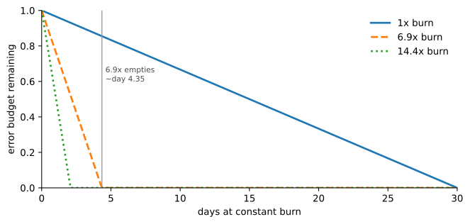
Paging on a single instantaneous burn is a bad trade: a high threshold misses slow leaks, a low one pages on harmless noise. The SRE Workbook’s answer is multiwindow alerting: require the burn to exceed a threshold over both a long and a short window at once (Beyer et al. 2018). The long window confirms the burn is significant; the short window makes the page both fire quickly and — crucially — clear quickly once the problem resolves.
# @save
def window_burn(bad_flags: list[float], slo_target: float) -> float:
    """Burn rate over one window from its per-slot bad fractions.

    Args:
        bad_flags: Per-slot bad fractions in the window.
        slo_target: The objective.

    Returns:
        The window's burn rate, zero for an empty window.
    """
    if not bad_flags:
        return 0.0
    return (sum(bad_flags) / len(bad_flags)) / (1 - slo_target)


def multiwindow_page(long_burn: float, short_burn: float, threshold: float = 14.4) -> bool:
    """Fire only when both windows exceed the threshold together.

    Requiring the long *and* the short window to agree is what buys precision:
    the long window rejects brief noise, and the short window lets the alert
    resolve itself minutes after the incident does instead of ringing for an
    hour.

    Args:
        long_burn: Burn over the long confirmation window.
        short_burn: Burn over the short reaction window.
        threshold: The multiple both windows must exceed.

    Returns:
        Whether to page.
    """
    return long_burn >= threshold and short_burn >= threshold
We drive the rule against a scripted bad deploy: a per-minute bad fraction that sits at a benign 0.001 until a deploy at minute 20 pushes it to 0.12 (a 24x burn) until it is reverted at minute 80. A trailing 30-minute window plays the long role and a 5-minute window the short one.
minutes = list(range(0, 130))
bad_series = [0.12 if 20 <= m < 80 else 0.001 for m in minutes]

def trailing_burn(series: list[float], end: int, window: int) -> float:
    return window_burn(series[max(0, end - window + 1): end + 1], 0.995)

rows = [(m, trailing_burn(bad_series, m, 30), trailing_burn(bad_series, m, 5)) for m in minutes]
combined = [m for m, lb, sb in rows if multiwindow_page(lb, sb)]
short_only = [m for m, lb, sb in rows if sb >= 14.4]
long_only = [m for m, lb, sb in rows if lb >= 14.4]
print(f"short window alone pages: minute {short_only[0]}..{short_only[-1]}")
print(f"long window alone pages:  minute {long_only[0]}..{long_only[-1]}")
print(f"combined rule pages:      minute {combined[0]}..{combined[-1]}")
short window alone pages: minute 22..81
long window alone pages: minute 37..91
combined rule pages: minute 37..81The short window alone would page from minute 22 — fast, but it would also fire on any brief blip. The combined rule waits until minute 37, when the long window confirms the burn is real, and stops at minute 81, minutes after the revert, because the short window drains even though the long one stays elevated to minute 91. Figure 27.4 shows the two burn curves and the region where the rule pages.
Show the code that draws this figure
fig, ax = plt.subplots(figsize=(7.2, 3.4))
ax.plot(minutes, [lb for _, lb, _ in rows], "-", linewidth=2, label="long (30-min) burn")
ax.plot(minutes, [sb for _, _, sb in rows], "--", linewidth=1.5, label="short (5-min) burn")
ax.axhline(14.4, color="0.5", linewidth=1)
ax.text(2, 15.6, "14.4x threshold", fontsize=8, color="0.3")
ax.axvspan(combined[0], combined[-1], color="#d9534f", alpha=0.15)
ax.text((combined[0] + combined[-1]) / 2, 26, "combined\npages here", fontsize=8,
        ha="center", color="#a33")
ax.set(xlabel="minute", ylabel="burn rate", xlim=(0, 129), ylim=(0, 28))
ax.legend(frameon=False, loc="upper right")
ax.spines[["top", "right"]].set_visible(False)
fig.tight_layout()
plt.show()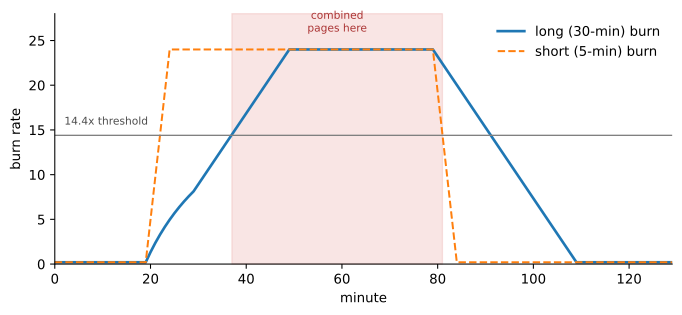
Low traffic complicates all of this: one failure can produce enormous burn on thin evidence, while a rare safety failure is too important to wait for volume. Use longer windows, event counts, and synthetic probes for the first, and say plainly which rule is SLO-budgeted and which is zero-tolerance — a distinction Section 27.6 makes executable.
27.5 Detect drift and decide a canary
Offline evaluation is controlled and reproducible; production traffic supplies the distribution, dependency, and interaction reality offline tests cannot. We use both without putting an expensive judge in the request path: sample eligible completed runs, redact content, and score asynchronously once the authoritative outcome is ready (the calibrated judge is Chapter 22’s). Then we watch for drift — a change in the live distribution relative to a reference — and the first mistake to avoid is trusting the fleet average. A single mean can stay green while it hides a per-slice collapse.
# @save
from statistics import mean


def drift_by_tenant(baseline: list[RunRecord], current: list[RunRecord],
                    threshold: float) -> dict[str, float]:
    """Return per-tenant score drops exceeding a threshold, hiding none in a mean.

    A fleet average is a weighted blend, so one tenant's improvement can mask
    another's regression. Comparing tenants separately is what surfaces the
    concentrated harm a single number launders away.

    Args:
        baseline: Reference-window records.
        current: Live-window records.
        threshold: The minimum mean drop worth alerting on.

    Returns:
        A mapping of tenant to score drop for tenants past the threshold.
    """
    def by_tenant(records: list[RunRecord]) -> dict[str, list[float]]:
        out: dict[str, list[float]] = {}
        for r in records:
            out.setdefault(r.tenant, []).append(r.score)
        return out

    base, live = by_tenant(baseline), by_tenant(current)
    alerts = {}
    for tenant in sorted(base.keys() & live.keys()):
        drop = mean(base[tenant]) - mean(live[tenant])
        if drop >= threshold:
            alerts[tenant] = round(drop, 6)
    return alerts
Suppose tenant A improves from 0.9 to 1.0 while tenant B falls from 0.9 to 0.4. The fleet mean drops only from 0.9 to 0.7 and sails over a coarse 0.6 threshold; tenant B has suffered a half-point regression.
baseline = [RunRecord(f"b{i}", "A", True, True, 1, 10, 1, 0.9) for i in range(20)] + \
           [RunRecord(f"b{i}", "B", True, True, 1, 10, 1, 0.9) for i in range(20)]
current = [RunRecord(f"c{i}", "A", True, True, 1, 10, 1, 1.0) for i in range(20)] + \
          [RunRecord(f"c{i}", "B", False, False, 0, 10, 1, 0.4) for i in range(20)]
print(f"fleet mean {mean(r.score for r in baseline):.2f} -> {mean(r.score for r in current):.2f}")
print("per-tenant alerts:", drift_by_tenant(baseline, current, 0.2))
fleet mean 0.90 -> 0.70
per-tenant alerts: {'B': 0.5}Figure 27.5 draws the trap: the fleet line stays above threshold while tenant B falls through the floor.
Show the code that draws this figure
series = {"tenant A": (0.9, 1.0), "tenant B": (0.9, 0.4), "fleet mean": (0.9, 0.7)}
styles = {"tenant A": ("#2a7f9e", "-"), "tenant B": ("#b13f3f", "-"), "fleet mean": ("0.35", "--")}
fig, ax = plt.subplots(figsize=(5.8, 3.4))
for name, (b, c) in series.items():
    color, ls = styles[name]
    ax.plot([0, 1], [b, c], ls, color=color, linewidth=2.2, marker="o")
    ax.text(1.02, c, name, fontsize=8, va="center", color=color)
ax.axhline(0.6, color="0.7", linewidth=1)
ax.text(0.02, 0.62, "0.6 alert threshold", fontsize=8, color="0.4")
ax.set(xticks=[0, 1], xlim=(0, 1.35), ylim=(0.3, 1.05), ylabel="mean score")
ax.set_xticklabels(["baseline", "current"])
ax.spines[["top", "right"]].set_visible(False)
fig.tight_layout()
plt.show()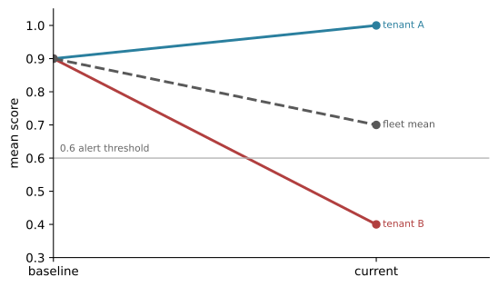
Detection is never instantaneous, and it is worth measuring the lag. A trailing-window detector smooths noise but pays for it in delay: the window must fill with post-shift data before its mean crosses. We feed a stream that shifts from 0.9 to 0.6 at sample 30 and measure how many samples pass before a 20-wide window notices.
# @save
from collections import deque


def streaming_drift_delay(reference_mean: float, stream: list[float],
                          window: int, threshold: float) -> int:
    """Return the sample index at which a trailing window first detects a drop.

    A wider window rejects noise but detects later, because its mean cannot
    cross the threshold until enough shifted samples have displaced the old
    ones — the detection delay is the price of the smoothing.

    Args:
        reference_mean: The pre-shift mean to compare against.
        stream: Incoming scores in order.
        window: Trailing-window width.
        threshold: The drop below reference that fires.

    Returns:
        The 1-based sample count at first detection, or -1 if never.
    """
    win: deque[float] = deque(maxlen=window)
    for index, score in enumerate(stream):
        win.append(score)
        if len(win) == window and (reference_mean - mean(win)) >= threshold:
            return index + 1
    return -1
The measured lag:
stream = [0.9] * 30 + [0.6] * 60
fired = streaming_drift_delay(0.9, stream, window=20, threshold=0.15)
print(f"shift at sample 30, detector fires at sample {fired} -> delay {fired - 30} samples")
shift at sample 30, detector fires at sample 40 -> delay 10 samplesTen samples of delay is not a bug; it is the window doing its job, and the number is what a runbook needs when it asks “how stale is our detection?” A difference is also not automatically harm: a product launch can create intentional input drift, and a score shift can come from a judge update rather than the agent, so a fired detector triggers investigation, not an automatic rollback.
That investigation often ends at a canary — a new release taking a slice of traffic beside the current one. Deciding whether to ship it is a two-proportion comparison, not an eyeball. We pool the two success rates, form the z-statistic, and gate on both significance and sample size.
# @save
def canary_decision(control_good: int, control_total: int, canary_good: int,
                    canary_total: int, min_count: int = 100, z_crit: float = 1.645) -> dict[str, Any]:
    """Decide ship / hold / rollback for a canary from a two-proportion test.

    A canary that looks worse might just be small, so the rule holds for more
    evidence below ``min_count``, rolls back only when the canary is
    *significantly* worse than control, and ships otherwise — the same
    discipline an A/B test uses, applied to a release gate.

    Args:
        control_good: Good journeys on the current release.
        control_total: Eligible journeys on control.
        canary_good: Good journeys on the canary.
        canary_total: Eligible journeys on the canary.
        min_count: Minimum canary sample before deciding.
        z_crit: One-sided critical value for "significantly worse".

    Returns:
        A decision with the z-statistic and both proportions.
    """
    p_control, p_canary = control_good / control_total, canary_good / canary_total
    if canary_total < min_count:
        return {"decision": "hold", "z": None, "p_control": p_control, "p_canary": p_canary}
    pooled = (control_good + canary_good) / (control_total + canary_total)
    se = math.sqrt(pooled * (1 - pooled) * (1 / control_total + 1 / canary_total))
    z = (p_canary - p_control) / se if se > 0 else 0.0
    decision = "rollback" if z <= -z_crit else "ship"
return {"decision": decision, "z": round(z, 2), "p_control": p_control, "p_canary": p_canary}print("bad release:", canary_decision(970, 1000, 900, 1000))
print("good release:", canary_decision(970, 1000, 965, 1000))
print("tiny sample :", canary_decision(970, 1000, 24, 25))bad release: {'decision': 'rollback', 'z': -6.35, 'p_control': 0.97, 'p_canary': 0.9}
good release: {'decision': 'ship', 'z': -0.63, 'p_control': 0.97, 'p_canary': 0.965}
tiny sample : {'decision': 'hold', 'z': None, 'p_control': 0.97, 'p_canary': 0.96}A canary at 90 percent against a 97 percent control is 6.35 standard errors worse — an unambiguous rollback. A 96.5 percent canary is within noise and ships. A 25-run canary, however tempting its 96 percent looks, holds for more evidence: shipping on it would be reading tea leaves. The canary-power arithmetic behind min_count is Chapter 22’s; the operational rule is that the gate refuses to decide without enough evidence.
27.6 Let evidence lower autonomy, and test it with chaos
An error-budget policy is executable governance: before the bad day, map evidence to automatic and human actions so the response is a lookup, not an argument. The policy is a pure function of the burn rate and one safety flag, which keeps it reviewable and testable.
# @save
def autonomy_action(burn: float, safety_violation: bool = False) -> str:
    """Map fleet evidence to a bounded runtime posture.

    Rising burn tightens autonomy step by step — ticket, review, read-only —
    so blast radius shrinks before anyone knows the cause. A safety violation
    is not on this ladder at all: it stops new effects regardless of burn,
    because safety is an invariant, not a budget you are allowed to spend.

    Args:
        burn: The current burn rate.
        safety_violation: Whether an invariant (not a quality target) broke.

    Returns:
        The runtime posture to enter.
    """
    if safety_violation:
        return "stop_new_effects"
    if burn >= 14.4:
        return "read_only_and_freeze_rollout"
    if burn >= 6.0:
        return "require_review_and_page"
    if burn >= 1.0:
        return "open_ticket"
    return "normal"
Walking the ladder from calm to crisis, with the safety flag as the last row:
for b, safety in [(0.2, False), (2.0, False), (6.9, False), (20.0, False), (0.1, True)]:
    print(f"burn={b:<5} safety={safety!s:<5} -> {autonomy_action(b, safety)}")
burn=0.2 safety=False -> normal
burn=2.0 safety=False -> open_ticket
burn=6.9 safety=False -> require_review_and_page
burn=20.0 safety=False -> read_only_and_freeze_rollout
burn=0.1 safety=True -> stop_new_effectsAt 6.9 times the fleet enters require_review_and_page; a safety flag at a mere 0.1 times still returns stop_new_effects. That last row is the load-bearing one: quality is a metric that can consume a budget, but an unauthorized cross-tenant disclosure or an unapproved irreversible effect is an invariant violation that triggers containment no matter how green the monthly average.
A policy is only worth its assertions if it survives real failure, which is what chaos engineering tests: state a measurable steady-state hypothesis, inject one realistic fault under a bounded blast radius, and check the invariant held (Basiri et al. 2016). It is not random production breakage. The sharpest agent drill targets the effect gap — the moment after a provider accepts an effect but before the worker records it. Our hypothesis: exactly one effect survives a worker kill in that gap. The mechanism that must make it true is an idempotency key (Chapter 26’s), so the drill runs the same retry with and without one.
# @save
def apply_effect_once(store: dict[str, Any], key: str, receipt: dict[str, Any]) -> tuple[dict[str, Any], bool]:
    """Apply an effect at most once per idempotency key.

    Keying the write on a stable idempotency token is what makes a retry after
    a crash safe: the second attempt finds the key already present and returns
    the first receipt instead of moving money twice.

    Args:
        store: The effect store keyed by idempotency token.
        key: The idempotency key for this action.
        receipt: The receipt to record on first application.

    Returns:
        The stored receipt and whether this call created a new effect.
    """
    if key in store:
        return store[key], False
    store[key] = receipt
    return receipt, True


def run_chaos_drill(use_idempotency_key: bool) -> int:
    """Kill a worker in the effect gap, retry, and count surviving effects.

    Args:
        use_idempotency_key: Whether the retry reuses a stable key.

    Returns:
        The number of distinct effects after the retry.
    """
    store: dict[str, Any] = {}
    for attempt in (1, 2):  # attempt 1 accepted then killed; attempt 2 is the retry
        key = "refund:A-17:v1" if use_idempotency_key else f"auto-token-{attempt}"
        apply_effect_once(store, key, {"attempt": attempt, "refunded_cents": 4999})
    return len(store)
The drill runs the same crash-and-retry twice, once with the idempotency key and once without it.
with_key = run_chaos_drill(True)
without_key = run_chaos_drill(False)
print(f"with idempotency key    -> {with_key} effect   (hypothesis holds)")
print(f"without idempotency key -> {without_key} effects  (invariant violated)")
assert with_key == 1
with idempotency key -> 1 effect (hypothesis holds)
without idempotency key -> 2 effects (invariant violated)The drill passes with the key and fails without it — a double refund conjured from one instruction. That failing run is the point: it names the exact control (the idempotency key) the invariant depends on, and it becomes a permanent test in Section 27.7. A chaos card names the hypothesis, the steady-state indicators, the blast radius, the abort condition, and the evidence retained; you start in a disposable environment and only graduate to a tiny production cohort when the abort conditions are proven.
27.7 Run the incident through both rollbacks
An incident begins when behavior threatens users or an invariant, not when the cause is known. Its lifecycle is detection, declaration, containment, diagnosis, recovery, then learning, and its most instructive property is that containment and recovery are different acts — as are the two kinds of rollback. Figure 27.6 separates them.
stateDiagram-v2
    [*] --> DETECT: alert, report, or audit mismatch
    DETECT --> DECLARE: classify severity, assign commander
    DECLARE --> CONTAIN: stop new admission and effects
    CONTAIN --> DIAGNOSE: compare release, tenant, tool, trajectory
    DIAGNOSE --> TECHNICAL: revert or repair the bundle
    DIAGNOSE --> BUSINESS: reconcile executed consequences
    TECHNICAL --> RECOVER
    BUSINESS --> RECOVER
    RECOVER --> VALIDATE: SLI, invariant, authoritative state
    VALIDATE --> RAMP: controlled restoration
    RAMP --> LEARN: blameless postmortem + regression test
    LEARN --> [*]
The kill switch must have defined semantics, because “disable the agent” can mean stop new journeys, cancel active model calls, prevent new tool calls, revoke effect credentials, or drain queues. The strong containment path stops new admissions and new consequential effects while preserving receipts and read-only diagnosis. But it cannot retract a message already sent or reverse a transfer already settled — and that limit is exactly why there are two rollbacks. A technical rollback changes future behavior: point traffic to the last-known-good bundle, revoke a tool, rebuild a poisoned index. A business rollback repairs consequences already produced: void a transaction, notify an affected user, rotate an exposed secret. Confusing them is how teams “resolve” an incident by reverting a deploy while a hundred wrong refunds sit unreconciled.
The metric that most often hides is the time before anyone noticed. We compute an incident’s timeline from its event log, and the number to stare at is the mean time to detect — the gap between the first harmful event and detection, during which harm compounds silently.
# @save
def incident_timeline(events: list[dict[str, Any]]) -> dict[str, int]:
    """Reduce an incident's event log to the intervals that grade the response.

    Mean time to detect — first harmful event to detection — is singled out
    because it is the interval where harm compounds unseen, and it is measured
    from the first *harmful effect*, not the first alert, so a late alarm
    cannot flatter the number.

    Args:
        events: Records with an integer ``t`` (minutes) and a ``kind``.

    Returns:
        Named intervals in minutes.
    """
    t = {e["kind"]: e["t"] for e in events}
    return {
        "mttd_min": t["detected"] - t["first_harmful"],
        "time_to_contain_min": t["contained"] - t["detected"],
        "harm_window_min": t["last_harmful_effect"] - t["first_harmful"],
        "technical_recovery_min": t["technical_recovered"] - t["detected"],
        "business_recovery_min": t["business_recovered"] - t["detected"],
    }
The scenario: at minute 0 a new retrieval connector begins producing outputs shaped like data exfiltration for one tenant; the general task-success chart stays green. The canary drift detector fires at minute 47. Containment revokes the connector at 52, the last harmful effect lands at 55, the bundle is reverted (technical recovery) at 70, and every affected record is reconciled (business recovery) at 190.
events = [
    {"t": 0, "kind": "first_harmful"},
    {"t": 47, "kind": "detected"},
    {"t": 52, "kind": "contained"},
    {"t": 55, "kind": "last_harmful_effect"},
    {"t": 70, "kind": "technical_recovered"},
    {"t": 190, "kind": "business_recovered"},
]
for name, value in incident_timeline(events).items():
    print(f"{name:24} {value}")
mttd_min 47
time_to_contain_min 5
harm_window_min 55
technical_recovery_min 23
business_recovery_min 143Forty-seven minutes of undetected harm dwarfs the five-minute containment, and the business rollback takes 143 minutes against the technical rollback’s 23 — the routine asymmetry that catches teams who declared victory at “the deploy is reverted.” Asynchronous outcome scoring, drift slices, and effect reconciliation are what shrink that 47-minute gap. Finally, a resolved incident earns a permanent test so the same failure cannot recur silently.
# @save
def as_regression_test(incident_id: str, invariant: str, probe: str) -> dict[str, str]:
    """Freeze a resolved incident into a permanent regression case.

    An incident that leaves only a postmortem can recur; one that leaves a
    runnable probe on the exact invariant it broke cannot recur silently,
    which is why "add the test" is the corrective action and "be more careful"
    is not.

    Args:
        incident_id: The incident identifier.
        invariant: The property that must hold forever after.
        probe: The runnable check that asserts it.

    Returns:
        A regression case wired to the release and chaos gates.
    """
    return {"case_id": f"regression::{incident_id}", "invariant": invariant,
            "probe": probe, "gate": "release + chaos"}
The incident above becomes a permanent case:
print(as_regression_test(
    "INC-1042",
    "no tool path bypasses the effect policy-enforcement point",
    "replay the exfiltration prompt; assert zero non-allowlisted egress receipts"))
{'case_id': 'regression::INC-1042', 'invariant': 'no tool path bypasses the effect policy-enforcement point', 'probe': 'replay the exfiltration prompt; assert zero non-allowlisted egress receipts', 'gate': 'release + chaos'}Success here is not naming the poisoned connector. It is that containment did not depend on that diagnosis, that missing sampled traces never hid the authoritative effect evidence, and that both rollbacks received an owner — the exact discipline the tabletop in Chapter 32’s failure game exercises without re-teaching.
27.8 Operate human review as a queue
Chapter 17 bound an approval to one action and Chapter 26 made the pause durable; operations must ensure a qualified person can actually decide in time, with real evidence, without being trained to click approve. That makes review a queue with measurable behavior, and the first thing to measure is whether the queue discriminates at all.
# @save
@dataclass(frozen=True)
class ApprovalRecord:
    """One review decision: what was decided and how long it took.

    Latency and decision together are what expose a rubber stamp — near-total
    approval reached in a fraction of a second is not oversight, it is a queue
    whose policy should either automate or supply harder cases.
    """

    action_id: str
    decision: str  # approve | deny | override | modify | abandon
    latency_s: float


def hitl_metrics(records: list[ApprovalRecord]) -> dict[str, Any]:
    """Measure whether a review queue oversees or merely rubber-stamps.

    A 99 percent approval rate reached in 0.2 seconds is flagged not because
    approving is wrong but because a person cannot weigh a consequential action
    that fast — the combined rate-and-latency signal catches the degenerate
    queue a raw approval count would call healthy.

    Args:
        records: Completed and abandoned review decisions.

    Returns:
        Approval, override, and abandonment rates, median decision time, and
        the rubber-stamp signal.
    """
    if not records:
        raise ValueError("approval records cannot be empty")
    completed = [r for r in records if r.decision != "abandon"]
    approvals = [r for r in completed if r.decision == "approve"]
    overrides = [r for r in completed if r.decision in {"override", "modify"}]
    latencies = sorted(r.latency_s for r in completed)
    n = len(latencies)
    median = latencies[n // 2] if n % 2 else (latencies[n // 2 - 1] + latencies[n // 2]) / 2
    approval_rate = len(approvals) / len(completed) if completed else 0.0
    return {
        "approval_rate": round(approval_rate, 4),
        "override_rate": round(len(overrides) / len(completed), 4) if completed else 0.0,
        "abandonment_rate": round((len(records) - len(completed)) / len(records), 4),
        "median_decision_s": median,
        "rubber_stamp_signal": approval_rate >= 0.98 and median < 1.0,
    }
Two queues make the signal concrete: one that approves 99 of 100 items in 0.2 seconds each, and one that spreads its decisions across approvals, denials, and modifications taking seconds to tens of seconds.
rubber = [ApprovalRecord(f"a{i}", "approve", 0.2) for i in range(99)] + \
         [ApprovalRecord("a99", "deny", 0.3)]
healthy = ([ApprovalRecord(f"h{i}", "approve", 8.0) for i in range(60)] +
           [ApprovalRecord(f"g{i}", "deny", 12.0) for i in range(20)] +
           [ApprovalRecord(f"m{i}", "modify", 20.0) for i in range(15)] +
           [ApprovalRecord(f"x{i}", "abandon", 0.0) for i in range(5)])
print("rubber-stamp queue:", hitl_metrics(rubber))
print("healthy queue     :", hitl_metrics(healthy))
rubber-stamp queue: {'approval_rate': 0.99, 'override_rate': 0.0, 'abandonment_rate': 0.0, 'median_decision_s': 0.2, 'rubber_stamp_signal': True}
healthy queue : {'approval_rate': 0.6316, 'override_rate': 0.1579, 'abandonment_rate': 0.05, 'median_decision_s': 8.0, 'rubber_stamp_signal': False}The first queue trips rubber_stamp_signal; the second, at a 63 percent approval rate with real override and abandonment, does not. Figure 27.7 separates them visually — a degenerate cluster against a healthy spread.
Show the code that draws this figure
import numpy as np

rng = np.random.default_rng(0)
levels = {"approve": 0, "deny": 1, "modify": 2}
fig, ax = plt.subplots(figsize=(7.0, 3.2))
for records, color, label in [(rubber, "#b13f3f", "rubber-stamp"), (healthy, "#2a7f9e", "healthy")]:
    pts = [r for r in records if r.decision in levels]
    xs = [r.latency_s for r in pts]
    ys = [levels[r.decision] + rng.uniform(-0.14, 0.14) for r in pts]
    ax.scatter(xs, ys, s=22, alpha=0.6, color=color, label=label)
ax.set(xlabel="decision latency (s)", yticks=[0, 1, 2], xlim=(-1, 24))
ax.set_yticklabels(["approve", "deny", "modify"])
ax.legend(frameon=False, loc="center right")
ax.spines[["top", "right"]].set_visible(False)
fig.tight_layout()
plt.show()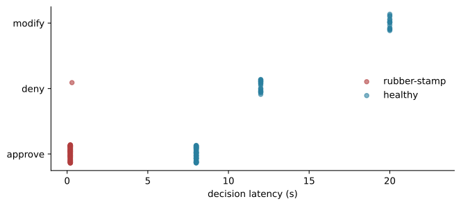
Behavior aside, a queue also needs enough people. Little’s Law gives the planning check: the average number of items in the system L equals the arrival rate \lambda times the average time in system W. Staffing is stable only when review capacity exceeds arrivals.
# @save
def queue_length(arrival_per_hr: float, service_time_hr: float) -> float:
    """Average items in the system by Little's Law, ``L = lambda * W``."""
    return arrival_per_hr * service_time_hr


def queue_stable(arrival_per_hr: float, reviewers: int, service_time_hr: float) -> bool:
    """Whether review capacity strictly exceeds the arrival rate.

    Args:
        arrival_per_hr: Review items arriving per hour.
        reviewers: Number of reviewers.
        service_time_hr: Average handling time per item in hours.

    Returns:
        True when the queue does not grow without bound.
    """
    return arrival_per_hr < reviewers / service_time_hr
At forty arrivals an hour and fifteen-minute reviews:
print(f"L = {queue_length(40, 0.25)} items in system (40/hr, 15-min reviews)")
print("stable with 12 reviewers?", queue_stable(40, 12, 0.25))
print("stable with  9 reviewers?", queue_stable(40, 9, 0.25))
L = 10.0 items in system (40/hr, 15-min reviews)
stable with 12 reviewers? True
stable with 9 reviewers? FalseForty arrivals an hour at fifteen minutes each keep ten items in flight and demand more than ten reviewers; nine cannot keep up and the queue grows without bound regardless of a beautiful SLA. During overload the failure mode to refuse is silently widening authority — a week-old approval must never release an action whose amount, destination, or policy changed while it waited. Lower autonomy instead, prioritize expiry and consequence, and preserve separation of duties. Reviewer wellbeing and the incentives around these numbers are Chapter 28’s.
27.9 Make telemetry private by construction
Telemetry is a second data product, and often a leakier one than the application: it outlives application state, reaches more operators and vendors, and copies prompts, tool arguments, and model output into indexes optimized for search. A tracing feature can become the breach. The durable rule is content off by default and redact before the span is created, not in the backend UI — because an exporter fans out to several systems and network buffers and collector logs may hold the secret before any server-side masking runs.
The naive redactor is a substring match on sensitive words, and it has a bug worth meeting head-on. A pattern matching token as a substring also matches the perfectly benign usage-metric key gen_ai.usage.input_tokens.
import re

buggy = re.compile(r"authorization|api[_-]?key|token|secret", re.IGNORECASE)
print("buggy pattern redacts 'gen_ai.usage.input_tokens'?",
      bool(buggy.search("gen_ai.usage.input_tokens")))
buggy pattern redacts 'gen_ai.usage.input_tokens'? TrueIn a chapter whose thesis is privacy-safe telemetry, a redactor that destroys the token counts — the numbers we need for cost and throughput — is a self-inflicted wound. The fix is to match whole dotted segments against an allowlist of secret names, so input_tokens never matches token, while a value scan still catches a bearer credential embedded in a string.
# @save
import hashlib
import re

SECRET_SEGMENTS = {"authorization", "api_key", "api-key", "apikey", "access_token",
                   "token", "secret", "password", "cookie", "set-cookie"}
BEARER = re.compile(r"(?i)bearer\s+[a-z0-9._~+/=-]+")


def _secret_key(key: str) -> bool:
    return key.rsplit(".", 1)[-1].strip().lower() in SECRET_SEGMENTS


def sanitize_attributes(attributes: dict[str, Any], capture_content: bool = False) -> dict[str, Any]:
    """Redact secrets and minimize identity and content before span creation.

    Secret-named fields are matched on whole dotted segments, not substrings,
    so ``input_tokens`` is never mistaken for a ``token`` secret — the exact
    false positive that would have deleted benign usage counts. Content is
    dropped unless explicitly captured, tenant ids become short surrogates,
    and bearer values are scrubbed even out of free-text error messages.

    Args:
        attributes: Raw span attributes.
        capture_content: Whether approved content capture is enabled.

    Returns:
        A sanitized copy safe to attach to a span.
    """
    cleaned: dict[str, Any] = {}
    for key, value in attributes.items():
        if _secret_key(key):
            cleaned[key] = "[REDACTED]"
        elif key in {"gen_ai.input.messages", "gen_ai.output.messages"} and not capture_content:
            cleaned[key] = "[CONTENT_DISABLED]"
        elif key == "app.tenant.id":
            cleaned[key] = hashlib.sha256(str(value).encode()).hexdigest()[:12]
        elif isinstance(value, str):
            cleaned[key] = BEARER.sub("Bearer [REDACTED]", value)
        else:
            cleaned[key] = value
    return cleaned
We hand it the hard cases at once: a secret header, a raw tenant id, a captured prompt, the benign token counts, and a bearer credential leaked into an error string.
attrs = {
    "authorization": "Bearer abc.secret",
    "app.tenant.id": "tenant-raw",
    "gen_ai.input.messages": "private prompt",
    "gen_ai.usage.input_tokens": 20000,
    "error.message": "request used Bearer xyz.123 to call the tool",
}
for key, value in sanitize_attributes(attrs).items():
    print(f"{key:28} {value!r}")
authorization '[REDACTED]'
app.tenant.id '08300f5d4179'
gen_ai.input.messages '[CONTENT_DISABLED]'
gen_ai.usage.input_tokens 20000
error.message 'request used Bearer [REDACTED] to call the tool'The header is redacted, the tenant becomes a stable surrogate that still joins incidents, the prompt is disabled, the bearer token is scrubbed from free text — and the token counts survive, exactly as intended. Regex is the last layer, not a privacy system: production needs structured parsing, allowlists, and tests over every instrumentation path, plus a telemetry data inventory with access control, residency, retention, and a deletion path. “Zero data retention” is a provider contract term, not an end-to-end property; it does not erase your own trace backend, crash dumps, or evaluation datasets, and it must be verified per endpoint and region. Deletion propagation into memories, embeddings, and adapters is Chapter 18’s; this section owns the operational job of finding and processing the telemetry copies.
Three privacy-enhancing technologies solve genuinely different problems, and senior literacy means knowing what each one costs — one concrete number apiece. Differential privacy bounds how much a single record can shift a released statistic, and its budget composes: several queries add their per-query \varepsilon.
# @save
def dp_epsilon(per_query_eps: list[float]) -> dict[str, float]:
    """Compose a differential-privacy budget and its worst-case leakage.

    Under basic composition the epsilons of successive queries add, and the
    total bounds how much one person's presence can change the output
    distribution by a factor of ``e**epsilon`` — so spending budget is literal,
    and after enough queries the guarantee is gone.

    Args:
        per_query_eps: Per-query epsilon spends.

    Returns:
        The total epsilon and its maximum likelihood ratio.
    """
    total = sum(per_query_eps)
    return {"total_epsilon": round(total, 4), "max_likelihood_ratio": round(math.exp(total), 2)}
Five queries at half a unit of budget each:
print("five queries at eps=0.5:", dp_epsilon([0.5] * 5))five queries at eps=0.5: {'total_epsilon': 2.5, 'max_likelihood_ratio': 12.18}Five queries at \varepsilon=0.5 spend a total budget of 2.5, meaning any one individual’s presence can change the output distribution by at most a factor of about 12 — and it does not hide raw inputs from the machine computing the statistic (Dwork and Roth 2014). Federated or on-device processing keeps raw examples decentralized and aggregates only summaries; a two-client weighted average shows the shape, and the caveat is that the summary can still leak and needs secure aggregation (McMahan et al. 2017).
# @save
def federated_average(client_updates: list[tuple[float, int]]) -> float:
    """Weight client summaries by example count without moving raw data.

    Each client contributes a summary and its sample size; the server forms a
    weighted mean, so raw examples never leave the device — though the summary
    itself can still leak and needs secure aggregation and, often, differential
    privacy on top.

    Args:
        client_updates: ``(summary, n_examples)`` per client.

    Returns:
        The example-weighted average.
    """
    total_n = sum(n for _, n in client_updates)
    if total_n == 0:
        raise ValueError("no client examples")
    return round(sum(update * n for update, n in client_updates) / total_n, 6)
Two clients contribute summaries weighted by their example counts:
print("federated average of A(0.9, n=100) and B(0.4, n=300):",
      federated_average([(0.9, 100), (0.4, 300)]))
federated average of A(0.9, n=100) and B(0.4, n=300): 0.525The global summary, 0.525, is pulled toward the larger client — computed with no raw record leaving either device. Confidential computing is the third: it protects data in use inside a hardware-attested enclave, so the attested boundary is the CPU package and its measured code, and the one thing it explicitly does not protect is the application logic itself — a prompt, an output, or an authorized-but-wrong recipient inside the enclave is still trusted. Choose a technology from the threat model and pair it with minimization and access control, never as a label.
NoteLandscape 2026 (dated)
Verify live: 2026-07-20. Appendix C owner: GenAI telemetry conventions, observability vendors, and provider retention terms. OpenTelemetry’s GenAI semantic conventions moved to a dedicated open-telemetry/semantic-conventions-genai repository and continue to evolve — pin the revision and version your attribute mapping. The observability landscape (Langfuse, Phoenix, LangSmith, Braintrust, Weave, OpenInference) and provider zero-data-retention, residency, and masking terms are fast-moving and contract-specific; a masking feature’s failure behavior in particular must be reviewed, not assumed. Maintain a counsel-reviewed vendor and jurisdiction matrix; never infer production privacy posture from this chapter’s dated examples.
The console now answers the two questions the opening dashboards could not — what the fleet is doing for users, and whether it is inside its declared budgets. We print it in one view, each field computed by a function above.
# @save
def operator_snapshot() -> dict[str, Any]:
    """Assemble the console's headline numbers from the chapter's own functions.

    Every field is produced by a function built earlier, so the snapshot is a
    real reduction of the fleet's runtime evidence — traces, indicators, burn,
    canary, chaos, and review — into the handful of numbers an operator reads
    first.

    Returns:
        A dictionary of the console's headline metrics.
    """
    spans, _ = emit_linked_run()
    b = burn_rate(9_655, 10_000, 0.995)
    reviews = [ApprovalRecord(f"a{i}", "approve", 0.2) for i in range(99)] + \
        [ApprovalRecord("a99", "deny", 0.3)]
    return {
        "spans": len(spans),
        "traces": len({s.context.trace_id for s in spans}),
        "diagnostic_trace_cost": trace_cost(spans),
        "slis": compute_slis(fixture_records()),
        "fleet_burn": round(b, 1),
        "days_to_exhaustion": round(days_to_exhaustion(30, 0.95, b), 1),
        "runtime_action": autonomy_action(b),
        "canary": canary_decision(970, 1000, 900, 1000)["decision"],
        "chaos_exactly_once": run_chaos_drill(True) == 1,
        "rubber_stamp": hitl_metrics(reviews)["rubber_stamp_signal"],
    }
import json
print(json.dumps(operator_snapshot(), indent=2, default=str)){
"spans": 5,
"traces": 2,
"diagnostic_trace_cost": 0.013,
"slis": {
"success_and_grounded_rate": 0.5,
"exactly_one_effect_rate": 0.75,
"p95_ttft_ms": 400,
"cost_per_successful_task": 0.028
},
"fleet_burn": 6.9,
"days_to_exhaustion": 4.1,
"runtime_action": "require_review_and_page",
"canary": "rollback",
"chaos_exactly_once": true,
"rubber_stamp": true
}
NoteIn the interview
Q. Your task-success dashboard is green at 96.5 percent, but users report the agent degrading. What do you look at, and what do you do? A green percentage is not a budget. Compute the burn rate against the actual SLO: 96.5 percent against a 99.5 percent target is a 6.9x burn that exhausts a 30-day budget in about four days. Then slice — a fleet mean hides per-tenant collapse — and reconcile authoritative effects, because a “success” that never changed state is not one. The action is to let burn lower autonomy (review-and-page here) while you diagnose, not to wait for the average to turn red. The trap is treating the aggregate as safe and reasoning from HTTP health instead of journey outcomes.
27.10 Summary
Operating an agent means joining infrastructure evidence to trajectory and outcome evidence on one journey identity. We built the console that does it: a real span tree with a durable pause as two linked traces; four channels so no store must be every truth; journey SLIs that demand grounding and charge failures to successes; error-budget burn paged by a precise multiwindow rule; per-tenant drift and a canary decision; an autonomy ladder tested by a chaos drill; an incident run through both rollbacks and frozen into a regression test; a review queue measured for rubber-stamping; and telemetry redacted before export. Chapter 28 turns this evidence into product decisions.
27.11 Exercises
- Extend the drift detector. Add a minimum sample count and a confidence interval to
drift_by_tenant, then construct a fleet in which the example-weighted average improves while one high-risk language slice regresses. Specify the alert your extended detector fires and the runtime action it should trigger. - Multiwindow against three patterns. Using
window_burnandmultiwindow_page, script three bad-event series: a 3-minute total outage, a sustained 2x burn for an hour, and intermittent 14.4x spikes. Design long/short windows and a threshold that page on the first and third but never on harmless low-volume noise, and report the minute each rule fires and clears. - Detection delay versus window width. Sweep the
windowargument ofstreaming_drift_delayfrom 5 to 50 on the same shifted stream and plot delay against width. Then add zero-mean noise to the post-shift scores and show how a narrow window trades a shorter delay for false alarms. What width would you choose for a safety-critical slice, and why? - Both rollbacks, with owners. Take the
incident_timelinescenario and write the two rollbacks explicitly:- the technical rollback (which bundle, which control-plane action, what health evidence gates the ramp), and
- the business rollback (which affected-object query, who owns notification, what proves reconciliation is complete). Then compute how the
mttd_minwould change if the canary detector fired at minute 20 instead of 47, and name one mechanism from Section 27.5 that would achieve it.
- Break and fix the redactor. Feed
sanitize_attributesa span carrying a bearer token in a tool-argument field, a full prompt on an error span, and a secret echoed inside model output. Show which ones survive, extend the sanitizer to catch them while keepinginput_tokensintact, and add a test that would fail on the original substring pattern. - Staff the queue. Given a week of
ApprovalRecord-style events with arrival timestamps, compute hourly arrival rate,queue_length, approval/override/abandonment by risk class, and the hours wherequeue_stableis false. Decide which risk class should be automated, which needs better evidence, and where the bottleneck is staffing rather than reviewer behavior. - Defend the four channels. A proposal wants to derive both invoices and the effect audit entirely from sampled traces to save a store. Using
trace_costand the sampling discussion in Section 27.2, write the rebuttal: name the sampling, exporter-loss, mutability, retention, and access-control failures the proposal creates, and state which single property of each channel makes it unfit for the other’s job.