flowchart LR
    GOAL["Language goal"] -->|task| POLICY(["Policy / VLA<br/>probabilistic proposal"])
    SENSOR["Sensors"] -->|observation| POLICY
    POLICY -->|proposed action| GATE{"Safety gate<br/>deterministic"}
    GATE -->|authorized| CTRL["Low-level controller"]
    GATE -->|deny| STOP["Hold safe state"]
    CTRL -->|torque / velocity| WORLD["Physical world<br/>irreversible effects"]
    WORLD -->|changed state| SENSOR
    WORLD -.->|state predicate| GRADE["Independent grader"]
31 World Models, VLA, and Embodied Agents
A warehouse robot sees a box near the edge of a table and receives “place the box on pallet three.” It predicts a grasp, the arm moves, and the box shifts under first contact. The next camera frame is no longer an independent query: it is evidence about a world the robot just changed. If the gripper closes two centimeters early, every later observation begins from the wrong state, and a fluent apology cannot un-crush the package. Acting in the physical world couples perception to consequence in a way a chatbot never faces.
We are now ready to build an embodied agent end to end on a toy we fully control, so that every claim is a number we can print: (i) a gridworld with a known nonlinear current, standing in for physical dynamics; (ii) a learned dynamics model — a small network trained from trajectories, whose one-step predictions are excellent; (iii) a planner that uses that model to choose actions, revealing that excellent one-step prediction is not the same as a model you can plan through; (iv) a vision-language-action policy that emits actions as discrete tokens, trained on demonstrations and executed in the loop; and (v) the safety seam — a reversibility gate that decides which proposals get physical authority. Along the way we place the 3D-representation bridge, the world-model landscape, simulators as infrastructure, and grounded skill selection where they belong. The reinforcement-learning machinery we lean on is Chapter 23’s; the approval loop is Chapter 16’s; Chapter 24 owns adversarial perception.
One honesty note before we start. Our environment is a two-dimensional box and our models train in seconds on a CPU, so every prediction, plan, and token is inspectable. A real robot swaps the box for contact-rich physics and the small networks for large ones, but the mechanisms on these pages — action tokens, compounding model error, receding-horizon feedback, the grader that reads state instead of the transcript — are exactly the mechanisms that survive the scale-up.
31.1 Acting closes a physical loop
An embodied agent wraps a policy around an environment whose state its actions change. Let x_t be the physical state, o_t the sensor observation, a_t the commanded action, and g the goal expressed in language. A compact closed-loop model is
x_{t+1}=f(x_t,a_t), \qquad o_t=h(x_t)+v_t, \qquad a_t=\pi(o_{\le t},g), \tag{31.1}
where f is the dynamics, h the observation process, v_t sensor noise, and \pi the policy. The policy sees observations, not x_t, and its action changes the distribution of the next observation. That coupling — the action is inside the loop that generates the next input — is the whole subject. Figure 31.1 separates the probabilistic proposal from the authority that executes it.
We need a concrete environment to make Equation 31.1 run. Our gridworld is a bounded box in which an action nudges the agent, but a state-dependent current — a smooth, invisible field — pushes it as well, the way friction, compliance, or a real draft would. The current is what makes the dynamics nonlinear and therefore worth learning: a model that ignores it is wrong in a way that matters.
# @save
import math

import numpy as np
import torch
import torch.nn as nn

torch.set_num_threads(4)

SIZE, MOVE, AMP = 6.0, 0.7, 0.40  # box side, action gain, current strength


def current(state: np.ndarray) -> np.ndarray:
    """Return the state-dependent drift at each position.

    The current is a smooth, bounded, nonlinear field — the "physics" a
    learned model must capture. Because it depends on *where* the agent is,
    a model that predicts only the average effect of an action (a straight
    nudge) is systematically wrong, and that error is what compounds when
    the model is rolled forward.

    Args:
        state: Positions with shape ``(..., 2)`` in the box ``[0, SIZE]``.

    Returns:
        Drift vectors with the same shape as ``state``.
    """
    x, y = state[..., 0], state[..., 1]
    return np.stack([AMP * np.sin(1.1 * y + 0.5),
                     AMP * np.sin(1.1 * x + 1.3)], axis=-1)


def true_step(state: np.ndarray, action: np.ndarray) -> np.ndarray:
    """Advance the true dynamics one step: nudge, drift, clip to the box.

    This is ``f`` from @eq-ch31-loop — the ground truth no policy sees
    directly. An action in ``[-1, 1]^2`` is scaled by ``MOVE``; the current
    adds a position-dependent push; the box clips the result.

    Args:
        state: Current positions, shape ``(..., 2)``.
        action: Commanded velocities in ``[-1, 1]``, shape ``(..., 2)``.

    Returns:
        Next positions, clipped into ``[0, SIZE]``.
    """
    action = np.clip(action, -1.0, 1.0)
    return np.clip(state + MOVE * action + current(state), 0.0, SIZE)
One worked step shows the current at work. From the center, commanding a pure rightward move does not travel a clean MOVE units in x: the current bends the path.
s0 = np.array([3.0, 3.0])
s1 = true_step(s0, np.array([1.0, 0.0]))
print("start   ", s0.round(3))
print("action  ", [1.0, 0.0], " commanded move +0.70 in x")
print("next    ", s1.round(3), " drift =", current(s0).round(3))
start [3. 3.]
action [1.0, 0.0] commanded move +0.70 in x
next [3.455 2.603] drift = [-0.245 -0.397]The commanded step was purely horizontal, yet the agent also slid in y, because the current at that position has a vertical component. A controller that models only “action moves me right” will mispredict every step by that drift. The engineering burden of embodiment is exactly this list of things below the model — reference frames, the current, contact limits, control rate — and the discipline that the model’s output never becomes an actuator command without passing the gate in Figure 31.1. We build up to that gate; first we must give the policy something to see and something to say.
31.2 Spatial grounding for action
Our gridworld hands the policy a clean position vector. A real robot must first build that state from pixels and depth, and the representation it chooses decides which questions it can answer. This bridge from 2D perception to action is a field of its own; we keep it to the one decision that matters for an agent, which is what a representation makes queryable and what it leaves out.
A point cloud is a set of sampled 3D positions, often carrying color or learned features; depth sensors produce them directly, and point encoders such as PointNet make unordered sets usable by a network (Qi et al. 2017). It answers “where is the nearest surface,” but raw points define neither watertight surfaces nor free space. A mesh joins points into faces and supports collision checking and clearance queries, at the cost of reconstructing clean topology from noisy scans. A neural radiance field learns a function from position and view direction to color and density, optimized for photorealistic novel views (Mildenhall et al. 2020), and 3D Gaussian splatting renders a cloud of anisotropic blobs fast and beautifully (Kerbl et al. 2023) — but a scene that renders well is not certified free of collisions. A scene graph takes the opposite tack, exposing entities and relations like mug ON table or gripper NEAR handle that a planner can query symbolically (Armeni et al. 2019). Figure 31.2 renders one small scene four ways and labels the query each serves and the safety fact each drops.
Show the code that draws this figure
import matplotlib.pyplot as plt

rng = np.random.default_rng(0)
fig, ax = plt.subplots(1, 4, figsize=(9.6, 2.7))
# table rectangle + a mug + gripper, shared layout
table = np.array([[0.5, 1.0], [3.5, 1.0], [3.5, 1.3], [0.5, 1.3]])
mug, grip = np.array([2.6, 1.55]), np.array([1.2, 2.4])

pts = np.vstack([rng.uniform([0.5, 1.0], [3.5, 1.3], (60, 2)),
                 rng.normal(mug, 0.12, (25, 2))])
ax[0].scatter(pts[:, 0], pts[:, 1], s=4, color="0.25")
ax[0].set_title("point cloud", fontsize=9)
ax[0].text(0.5, 0.05, "nearest surface / pose\nmisses: free space",
           transform=ax[0].transAxes, ha="center", fontsize=7)

ax[1].fill(table[:, 0], table[:, 1], color="0.7")
ax[1].add_patch(plt.Circle(mug, 0.22, color="0.4"))
ax[1].set_title("mesh / SDF", fontsize=9)
ax[1].text(0.5, 0.05, "collision / clearance\nmisses: appearance",
           transform=ax[1].transAxes, ha="center", fontsize=7)

occ = np.zeros((8, 10))
occ[2, 1:8] = 1
occ[3, 5] = 1
ax[2].imshow(occ, cmap="Greys", origin="lower", extent=(0, 4, 0, 3.2))
ax[2].set_title("occupancy voxels", fontsize=9)
ax[2].text(0.5, 0.05, "free vs occupied\nmisses: object identity",
           transform=ax[2].transAxes, ha="center", fontsize=7)

nodes = {"table": (1.8, 1.15), "mug": (2.6, 1.9), "gripper": (1.0, 2.4)}
for a_, b_ in [("mug", "table"), ("gripper", "mug")]:
    ax[3].plot(*zip(nodes[a_], nodes[b_]), color="0.5", lw=1)
for name, (x, y) in nodes.items():
    ax[3].scatter([x], [y], s=220, color="0.85", edgecolor="0.2", zorder=3)
    ax[3].text(x, y, name, ha="center", va="center", fontsize=6.5, zorder=4)
ax[3].set_title("scene graph", fontsize=9)
ax[3].text(0.5, 0.05, "symbolic relations\nmisses: contact geometry",
           transform=ax[3].transAxes, ha="center", fontsize=7)

for a in ax:
    a.set_xticks([]); a.set_yticks([]); a.set_xlim(0, 4); a.set_ylim(0, 3.4)
fig.tight_layout()
plt.show()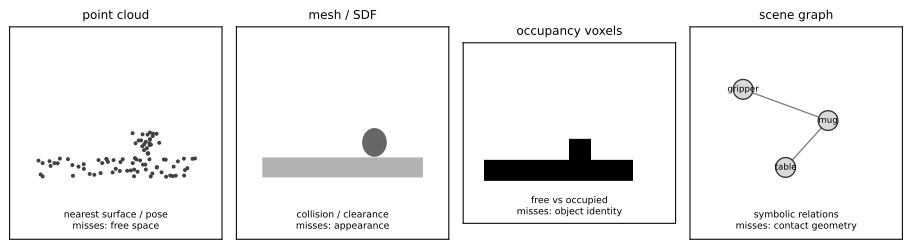
The lesson is not that one representation wins. It is that “renders well” and “safe to plan through” are different contracts, and a production stack usually fuses several — depth for geometry, a scene graph for task-level identity, learned features for the policy — plus the robot’s own proprioception, its joint positions and velocities. Our gridworld collapses all of this into a position because we want the rest of the loop under a microscope. With state in hand, the policy must produce an action, and the interesting question is what shape that action takes.
31.3 Actions as tokens
A transformer already knows how to emit tokens. The core idea behind the vision-language-action (VLA) family is to make robot actions look like tokens too, so that a model pretrained on web text and images can be fine-tuned to end its sequence with control commands instead of words (Brohan et al. 2022, 2023). Concretely, normalize each action coordinate to [-1,1], split that range into K bins, and emit the bin index.
q_j=\operatorname{round}\!\left(\frac{a_j+1}{2}(K-1)\right), \qquad \hat a_j=\frac{2 q_j}{K-1}-1 . \tag{31.2}
Here q_j\in\{0,\dots,K-1\} is the token and \hat a_j the value it decodes to. Rounding to the nearest bin center costs at most half a bin, so the worst-case per-coordinate error is {(K-1)}^{-1} — with K=256, about 0.0039.
# @save
def tokenize_action(action: np.ndarray, bins: int = 256) -> np.ndarray:
    """Quantize a normalized action into per-dimension integer tokens.

    Implements @eq-ch31-codec: each coordinate, assumed already normalized
    to ``[-1, 1]``, is mapped to its nearest of ``bins`` bin indices. The
    codec is dimension-agnostic — a 2-D gridworld velocity or a 7-DoF arm
    command tokenizes the same way.

    Args:
        action: Coordinates in ``[-1, 1]``, any length.
        bins: Vocabulary size per coordinate (at least 2).

    Returns:
        Integer tokens in ``[0, bins)``, one per coordinate.

    Raises:
        ValueError: If ``bins < 2`` or any coordinate leaves ``[-1, 1]``.
    """
    a = np.asarray(action, dtype=float)
    if bins < 2 or np.any(np.abs(a) > 1.0 + 1e-9):
        raise ValueError("need bins >= 2 and coordinates normalized to [-1, 1]")
    return np.rint((a + 1.0) * (bins - 1) / 2.0).astype(int)


def detokenize_action(tokens: np.ndarray, bins: int = 256) -> np.ndarray:
    """Map action tokens back to bin-center values in ``[-1, 1]``.

    The inverse of :func:`tokenize_action`, up to the half-bin rounding the
    forward map cannot undo.

    Args:
        tokens: Integer tokens in ``[0, bins)``.
        bins: Vocabulary size per coordinate.

    Returns:
        Decoded coordinates in ``[-1, 1]``.
    """
    return 2.0 * np.asarray(tokens, dtype=float) / (bins - 1) - 1.0


def roundtrip_error(action: np.ndarray, bins: int = 256) -> float:
    """Return the worst-coordinate error from one tokenize/detokenize pass."""
    a = np.asarray(action, dtype=float)
    return float(np.max(np.abs(a - detokenize_action(tokenize_action(a, bins), bins))))
A robot action is usually seven numbers — three for translation, three for rotation, one for the gripper. Tokenizing a sample 7-DoF command and reading it back shows the codec and its bound in one line:
sample = np.array([0.30, -0.55, 0.80, -0.10, 0.05, -0.95, 1.0])  # 3 xyz, 3 rot, 1 grip
print("tokens        ", tokenize_action(sample).tolist())
print("max round-trip", round(roundtrip_error(sample), 5), " bound 1/255 =", round(1 / 255, 5))
tokens [166, 57, 230, 115, 134, 6, 255]
max round-trip 0.00392 bound 1/255 = 0.00392The round-trip error sits exactly at the {(K-1)}^{-1} bound. But that bound is only about the codec. A mismatched convention — meters versus normalized deltas, open-positive versus close-positive gripper — produces perfectly valid tokens that command the wrong motion by orders of magnitude. The durable rule is to version the action contract with the checkpoint: coordinate order, frame, units, bounds, normalization statistics, chunk length, control rate, gripper sign. A VLA whose weights load but whose normalizer is lost is not deployable.
Per-dimension tokens are simple but verbose: a smooth trajectory of many timesteps becomes a long token string that is slow to decode. FAST observed that smooth action chunks compress well in the frequency domain — run a discrete cosine transform, keep the low-order coefficients, and tokenize those (Pertsch et al. 2025). Figure 31.3 makes both ideas visible: the quantization grid for one coordinate, and a 16-step chunk reconstructed from a handful of cosine coefficients.
# @save
def dct_ii(x: np.ndarray) -> np.ndarray:
    """Return the DCT-II frequency coefficients of a 1-D signal.

    A smooth action chunk concentrates its energy in the first few
    coefficients, which is exactly why frequency-domain action tokenization
    can represent a long chunk with a short token string.

    Args:
        x: The signal (an action chunk), shape ``(n,)``.

    Returns:
        Coefficients ordered low to high frequency, shape ``(n,)``.
    """
    n = len(x)
    basis = np.cos(np.pi * (2 * np.arange(n)[:, None] + 1) * np.arange(n)[None, :] / (2 * n))
    return basis.T @ x


def idct_ii(coef: np.ndarray) -> np.ndarray:
    """Reconstruct a signal from DCT-II coefficients (inverse of :func:`dct_ii`).

    Zeroing the high-frequency tail before calling this is the lossy
    compression step FAST exploits.

    Args:
        coef: Coefficients, shape ``(n,)``; zero the tail to compress.

    Returns:
        The reconstructed signal, shape ``(n,)``.
    """
    n = len(coef)
    basis = np.cos(np.pi * (2 * np.arange(n)[:, None] + 1) * np.arange(n)[None, :] / (2 * n))
    weight = np.full(n, 2.0)
    weight[0] = 1.0
    return (basis * (weight * coef)[None, :]).sum(1) / n
steps = np.linspace(0, 1, 16)
chunk = 0.8 * np.sin(2 * np.pi * steps) + 0.1 * steps # a smooth 16-step action chunk
coef = dct_ii(chunk)
for keep in (2, 4, 6):
trimmed = coef.copy()
trimmed[keep:] = 0.0
rmse = float(np.sqrt(np.mean((idct_ii(trimmed) - chunk) ** 2)))
print(f"keep {keep:>1} of 16 coeffs -> {16 / keep:.1f}x fewer tokens, reconstruction RMSE {rmse:.4f}")keep 2 of 16 coeffs -> 8.0x fewer tokens, reconstruction RMSE 0.3482
keep 4 of 16 coeffs -> 4.0x fewer tokens, reconstruction RMSE 0.0811
keep 6 of 16 coeffs -> 2.7x fewer tokens, reconstruction RMSE 0.0373Four coefficients reproduce the sixteen-step chunk with root-mean-square error 0.081 — a four-fold shorter token string for a small, controllable loss.
Show the code that draws this figure
fig, ax = plt.subplots(1, 2, figsize=(8.4, 3.0))
K = 13
centers = detokenize_action(np.arange(K), K)
ax[0].vlines(centers, 0, 1, color="0.8")
ax[0].plot([0.31], [0.5], "o", color="0.1")
snapped = detokenize_action(tokenize_action(np.array([0.31]), K), K)[0]
ax[0].plot([snapped], [0.5], "s", color="0.45")
ax[0].annotate(f"0.31 -> bin {int(tokenize_action(np.array([0.31]), K)[0])} ({snapped:.2f})",
               (0.31, 0.5), (0.0, 0.75), fontsize=8, ha="center")
ax[0].set(xlim=(-1.05, 1.05), ylim=(0, 1), yticks=[], xlabel="normalized coordinate")
ax[0].set_title(f"quantization ({K} bins)", fontsize=9)

trimmed = coef.copy(); trimmed[4:] = 0.0
ax[1].plot(steps, chunk, "o", color="0.2", ms=4, label="raw chunk (16 tokens)")
ax[1].plot(steps, idct_ii(trimmed), "-", color="0.45", label="4 DCT coeffs")
ax[1].set(xlabel="step in chunk", ylabel="action value")
ax[1].legend(fontsize=8)
ax[1].set_title("FAST-style compression", fontsize=9)
fig.tight_layout()
plt.show()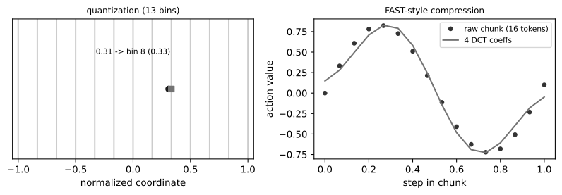
RT-2 placed action tokens in a vision-language model’s own vocabulary so web-scale semantics could transfer into control; OpenVLA released an open-weight model of that shape whose processor, prompt, and action call are inspectable (Kim et al. 2024); the \pi-series added a continuous action expert beneath the language model for high-rate control (Black et al. 2024). On real hardware the call looks like the sketch below — we show it but do not run it, because it needs a checkpoint and a GPU.
# Illustrative: the real OpenVLA-style call (needs a checkpoint + GPU; not run here).
from transformers import AutoModelForVision2Seq, AutoProcessor
from PIL import Image

processor = AutoProcessor.from_pretrained("openvla/openvla-7b", trust_remote_code=True)
model = AutoModelForVision2Seq.from_pretrained("openvla/openvla-7b").to("cuda:0")

prompt = "In: What action should the robot take to put the eggplant in the basket?\nOut:"
inputs = processor(prompt, Image.fromarray(agentview_image)).to("cuda:0")
action = model.predict_action(**inputs, unnorm_key="bridge_orig", do_sample=False)  # 7 numbers
The shape is identical to ours: an image and an instruction go in, tokens come out, and a decoder turns those tokens into a 7-DoF command. We now build the small version and run it.
31.4 A language-conditioned policy in the gridworld
Our policy consumes an observation — the agent position and the goal position, standing in for fused vision-language features — and emits a two-token action, one bin per coordinate. To have demonstrations to imitate, we need an expert. Because our current is known to us (though not to any learned model), we can write a clean feedback-linearizing controller: to land at the goal, command the move that cancels the drift and covers the gap.
# @save
def expert_action(state: np.ndarray, goal: np.ndarray) -> np.ndarray:
    """Return the demonstration controller's action toward ``goal``.

    Because the true current is known here, the expert inverts it: it asks
    for the nudge that, added to the drift, lands on the goal, then clips to
    the actuator range. This produces clean, near-optimal demonstrations for
    the policy to imitate — the toy stand-in for a teleoperator or a scripted
    oracle on a real robot.

    Args:
        state: Current position, shape ``(2,)``.
        goal: Target position, shape ``(2,)``.

    Returns:
        A demonstration action in ``[-1, 1]^2``.
    """
    state, goal = np.asarray(state, float), np.asarray(goal, float)
    return np.clip((goal - state - current(state)) / MOVE, -1.0, 1.0)


def collect_demos(n_pairs: int, seed: int, horizon: int = 30, tol: float = 0.25):
    """Roll the expert through random start/goal pairs and log (obs, action).

    Each observation is ``[x, y, goal_x, goal_y]``; each label is the
    expert's continuous action there. The dataset is exactly the states the
    *expert* visits — a coverage property that matters for imitation, as
    @sec-ch23 showed.

    Args:
        n_pairs: Number of start/goal episodes to demonstrate.
        seed: Seed for the start/goal sampler.
        horizon: Maximum steps per demonstration.
        tol: Distance at which the goal counts as reached.

    Returns:
        ``(obs, acts)`` float arrays of shape ``(N, 4)`` and ``(N, 2)``.
    """
    rng = np.random.default_rng(seed)
    obs, acts = [], []
    made = 0
    while made < n_pairs:
        s = rng.uniform(0.5, SIZE - 0.5, size=2)
        g = rng.uniform(0.5, SIZE - 0.5, size=2)
        if np.linalg.norm(s - g) < 2.0:
            continue
        for _ in range(horizon):
            a = expert_action(s, g)
            obs.append([s[0], s[1], g[0], g[1]])
            acts.append(a)
            s = true_step(s, a)
            if np.linalg.norm(s - g) <= tol:
                break
        made += 1
    return np.asarray(obs, np.float32), np.asarray(acts, np.float32)
The policy is autoregressive over the two action tokens: it predicts the first coordinate’s bin from the observation, then the second coordinate’s bin from the observation and the first token. This is the same factorization RT-2 places inside a transformer, p(a\mid o)=p(q_0\mid o)\,p(q_1\mid o,q_0), shrunk to a network that trains in a few seconds.
# @save
ACTION_BINS = 21  # bins per action coordinate for the policy


class ActionTokenPolicy(nn.Module):
    """A tiny autoregressive vision-language-action policy.

    An observation encoder produces a feature vector (the stand-in for a
    VLA's fused image-and-language embedding); action coordinates are then
    decoded one token at a time, each conditioned on the observation and the
    tokens already emitted. This is the actions-as-tokens mechanism of
    RT-2/OpenVLA at teaching scale: a real VLA replaces the encoder with a
    vision-language transformer and predicts more tokens, but the
    autoregressive action factorization is the same.
    """

    def __init__(self, dim: int = 64, bins: int = ACTION_BINS):
        super().__init__()
        self.bins = bins
        self.enc = nn.Sequential(nn.Linear(4, dim), nn.GELU(),
                                 nn.Linear(dim, dim), nn.GELU(), nn.Linear(dim, dim))
        self.pos = nn.Parameter(torch.zeros(2, dim))
        self.tok = nn.Embedding(bins, dim)
        self.head = nn.Sequential(nn.GELU(), nn.Linear(dim, bins))

    def logits(self, obs: torch.Tensor, prev: torch.Tensor | None, pos: int) -> torch.Tensor:
        """Return next-token logits at action position ``pos`` (0 or 1).

        Args:
            obs: Observations ``[x, y, goal_x, goal_y]``, shape ``(B, 4)``.
            prev: The previous action token, or ``None`` at position 0.
            pos: Which action coordinate is being decoded.

        Returns:
            Logits over the ``bins`` action tokens, shape ``(B, bins)``.
        """
        h = self.enc(obs / SIZE) + self.pos[pos]
        if prev is not None:
            h = h + self.tok(prev)
        return self.head(h)

    @torch.no_grad()
    def act(self, obs_np) -> np.ndarray:
        """Greedily decode both action tokens and return a continuous action."""
        obs = torch.as_tensor(np.atleast_2d(obs_np), dtype=torch.float32)
        t0 = self.logits(obs, None, 0).argmax(-1)
        t1 = self.logits(obs, t0, 1).argmax(-1)
        toks = torch.stack([t0, t1], -1).numpy()[0]
        return detokenize_action(toks, self.bins)


def train_policy(seed: int = 0, steps: int = 1500):
    """Behavior-clone the action-token policy from expert demonstrations.

    The loss is cross-entropy on both action tokens with teacher forcing —
    the second token is trained against the *true* first token, exactly the
    next-token objective from @sec-ch02, now over action bins.

    Args:
        seed: Seeds demonstrations, initialization, and batching.
        steps: Number of gradient steps.

    Returns:
        ``(policy, obs, acts)``: the trained policy and its training data.
    """
    torch.manual_seed(seed)
    obs, acts = collect_demos(260, seed)
    obs_t = torch.as_tensor(obs)
    tokens = torch.as_tensor(tokenize_action(acts, ACTION_BINS), dtype=torch.long)
    policy = ActionTokenPolicy()
    opt = torch.optim.Adam(policy.parameters(), lr=3e-3)
    ce = nn.CrossEntropyLoss()
    gen = torch.Generator().manual_seed(seed)
    for _ in range(steps):
        idx = torch.randint(0, obs_t.shape[0], (256,), generator=gen)
        o, tk = obs_t[idx], tokens[idx]
        opt.zero_grad()
        loss = ce(policy.logits(o, None, 0), tk[:, 0]) + ce(policy.logits(o, tk[:, 0], 1), tk[:, 1])
        loss.backward()
        opt.step()
    return policy, obs, acts
Training is a behavior-cloning loop; we then check how faithfully it reproduces the expert’s tokens, and — separately — a single decoded action.
policy, demo_obs, demo_acts = train_policy()
targets = tokenize_action(demo_acts, ACTION_BINS)
with torch.no_grad():
    p0 = policy.logits(torch.as_tensor(demo_obs), None, 0).argmax(-1).numpy()
    p1 = policy.logits(torch.as_tensor(demo_obs), torch.as_tensor(targets[:, 0]), 1).argmax(-1).numpy()
print("demonstrations       ", len(demo_obs))
print("within-1-bin accuracy", round(float((np.abs(p0 - targets[:, 0]) <= 1).mean()), 2),
      round(float((np.abs(p1 - targets[:, 1]) <= 1).mean()), 2))
obs_demo = [3.0, 3.0, 3.2, 2.9]
print("obs", obs_demo, "-> policy", policy.act(obs_demo).round(3).tolist(),
      " expert", expert_action(obs_demo[:2], obs_demo[2:]).round(3).tolist())
demonstrations 1279
within-1-bin accuracy 0.97 0.97
obs [3.0, 3.0, 3.2, 2.9] -> policy [0.6, 0.4] expert [0.635, 0.425]The policy matches the expert to within one action bin about 0.97 of the time on both coordinates, and the single decoded action tracks its target closely. But the tokens are quantized to a tenth of the range, so every commanded action is still slightly off. The honest question is whether that per-step slack drives the robot to the goal or accumulates into failure. We run it closed-loop: at each step, tokenize the observation, decode an action, take a true step, repeat.
# @save
def run_vla_episode(policy, start, goal, horizon: int = 30, tol: float = 0.6):
    """Drive one closed-loop episode with the token policy; grade final state.

    Args:
        policy: An object with ``act(obs) -> action``.
        start: Start position, shape ``(2,)``.
        goal: Goal position, shape ``(2,)``.
        horizon: Step budget.
        tol: Success distance to the goal.

    Returns:
        ``(reached, path)``: whether the goal was reached and the trajectory.
    """
    s = np.asarray(start, float)
    path = [s.copy()]
    for _ in range(horizon):
        s = true_step(s, policy.act([s[0], s[1], goal[0], goal[1]]))
        path.append(s.copy())
        if np.linalg.norm(s - goal) <= tol:
            return True, np.asarray(path)
    return False, np.asarray(path)


def vla_success(policy, n: int = 40, seed: int = 5):
    """Fraction of random start/goal episodes the policy solves closed-loop.

    Args:
        policy: A policy with an ``act(obs) -> action`` method.
        n: Number of random start/goal episodes to evaluate.
        seed: Seed for the start/goal sampler.

    Returns:
        ``(rate, paths)``: the success fraction and each episode's trajectory.
    """
    rng = np.random.default_rng(seed)
    wins, paths = 0, []
    for _ in range(n):
        s = rng.uniform(0.5, SIZE - 0.5, size=2)
        g = rng.uniform(0.5, SIZE - 0.5, size=2)
        if np.linalg.norm(s - g) < 2.0:
            g = np.clip(g + 2.5, 0.5, SIZE - 0.5)
        reached, path = run_vla_episode(policy, s, g)
        wins += reached
        paths.append((path, g, reached))
    return wins / n, paths
rate, paths = vla_success(policy)
print("closed-loop success rate:", rate)closed-loop success rate: 1.0Every episode reaches its goal, even though each per-step action is quantized and slightly off the expert’s. The slack does not matter because the loop is closed: a small error this step is corrected by the next observation. Figure 31.4 shows a handful of these trajectories curving toward their goals — and that same forgiveness is about to become the central lesson of the chapter, in a setting where it does not save us.
Show the code that draws this figure
fig, ax = plt.subplots(figsize=(4.6, 4.4))
for path, goal, reached in paths[:8]:
    ax.plot(path[:, 0], path[:, 1], "-", lw=1.3, alpha=0.8)
    ax.plot(path[0, 0], path[0, 1], "o", color="0.3", ms=6)
    ax.plot(goal[0], goal[1], "*", color="0.1", ms=12)
ax.set(xlim=(0, SIZE), ylim=(0, SIZE), xlabel="x", ylabel="y")
ax.set_title("action-token policy, closed loop", fontsize=10)
fig.tight_layout()
plt.show()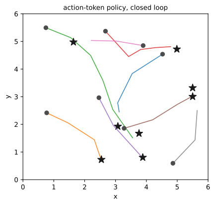
Two extensions matter at scale and both are contracts, not model sizes. Cross-embodiment training pools data from robots with different arms and action spaces; a shared policy emits a canonical action z_t and a per-robot adapter maps it to that robot’s command, u_t^{(e)}=A_e(z_t) — language names the task but does not align frames or gripper dynamics (Open X-Embodiment Collaboration 2024). And the slow-semantic/fast-action split of recent systems runs a large model at low rate to interpret the scene while a small expert emits dense control, which demands a handoff contract: the fast path must know when its instruction is stale.
NoteLandscape 2026 (dated)
Verify live: 2026-07-20. Appendix C owns the version roster. On the VLA side, Physical Intelligence’s \pi-series, NVIDIA’s GR00T, Figure’s Helix, and Google DeepMind’s Gemini Robotics are the frequently-cited families; on the world-model side, DeepMind’s Genie 3, Dreamer 4, Meta’s V-JEPA 2, and NVIDIA’s Cosmos foundation models. These names, their action rates, licenses, and hardware requirements move quarterly; recheck the primary research pages and active benchmark repositories before making any deployment claim. The mechanisms in this chapter — action tokens, compounding error, receding feedback, independent grading — outlast every name in this box.
31.5 Learning a world model
Our token policy maps observation straight to action. A world model instead learns how the environment itself changes — the transition f — optionally conditioned on the action. Written with a learned latent state z_t=E(o_{\le t}),
z_{t+1}\sim p_\theta(z_{t+1}\mid z_t,a_t), \qquad \hat o_{t+1}\sim p_\theta(o_{t+1}\mid z_{t+1}), \tag{31.3}
and for planning the first relation is load-bearing: it must be action-conditioned. A video predictor trained only to extrapolate likely footage learns that a gripper usually moves toward a cup, yet cannot answer what happens if it approaches from an unusual angle. In our gridworld the state is already the observation, so we learn the transition directly: a small network that predicts the delta s_{t+1}-s_t from the state and action.
# @save
def collect_transitions(n: int, seed: int):
    """Sample random (state, action, delta) transitions from the true dynamics.

    Random exploration is the simplest data engine: uniform states, uniform
    actions, and the resulting state change. Predicting the *delta* rather
    than the next state lets the model focus on the effect of the action and
    the current, which is where all the nonlinearity lives.

    Args:
        n: Number of transitions.
        seed: Seed for states and actions.

    Returns:
        ``(states, actions, deltas)`` float32 arrays.
    """
    rng = np.random.default_rng(seed)
    s = rng.uniform(0, SIZE, size=(n, 2))
    a = rng.uniform(-1, 1, size=(n, 2))
    return s.astype(np.float32), a.astype(np.float32), (true_step(s, a) - s).astype(np.float32)


class Dynamics(nn.Module):
    """A tiny action-conditioned dynamics model: (state, action) -> delta.

    This is $p_\\theta$ from @eq-ch31-wm made deterministic and small. It is
    the object we will plan through — and the object whose one-step accuracy
    turns out not to guarantee that plans through it succeed.
    """

    def __init__(self, hidden: int = 96):
        super().__init__()
        self.net = nn.Sequential(nn.Linear(4, hidden), nn.Tanh(),
                                 nn.Linear(hidden, hidden), nn.Tanh(),
                                 nn.Linear(hidden, 2))

    def forward(self, s: torch.Tensor, a: torch.Tensor) -> torch.Tensor:
        """Predict the state delta for states ``s`` and actions ``a``."""
        return self.net(torch.cat([s / SIZE, a], dim=-1))

    @torch.no_grad()
    def step(self, s: np.ndarray, a: np.ndarray) -> np.ndarray:
        """Advance one step under the model, clipping to the box like reality."""
        st = torch.as_tensor(np.atleast_2d(s), dtype=torch.float32)
        at = torch.as_tensor(np.atleast_2d(a), dtype=torch.float32)
        nxt = np.clip(np.atleast_2d(s) + self.forward(st, at).numpy(), 0.0, SIZE)
        return nxt.reshape(np.shape(s))


def train_dynamics(n_trans: int, seed: int, steps: int) -> Dynamics:
    """Fit a :class:`Dynamics` model by MSE on sampled transitions.

    Args:
        n_trans: Size of the transition dataset (the data budget).
        seed: Seeds data, initialization, and batching.
        steps: Gradient steps.

    Returns:
        The trained model.
    """
    torch.manual_seed(seed)
    s, a, d = collect_transitions(n_trans, seed)
    s, a, d = map(torch.as_tensor, (s, a, d))
    model = Dynamics()
    opt = torch.optim.Adam(model.parameters(), lr=3e-3)
    loss_fn = nn.MSELoss()
    gen = torch.Generator().manual_seed(seed)
    for _ in range(steps):
        idx = torch.randint(0, s.shape[0], (256,), generator=gen)
        opt.zero_grad()
        loss_fn(model(s[idx], a[idx]), d[idx]).backward()
        opt.step()
    return model
We train two models on purpose: a well-fit one from 8,000 transitions, and a deliberately under-fit one from just 40. Their one-step accuracy on held-out transitions is the number a demo would show off.
good = train_dynamics(8000, seed=0, steps=2500)
weak = train_dynamics(40, seed=1, steps=150)

s_te, a_te, d_te = collect_transitions(3000, seed=99)
with torch.no_grad():
    err_good = np.sqrt(((good(torch.as_tensor(s_te), torch.as_tensor(a_te)).numpy() - d_te) ** 2).sum(-1))
    err_weak = np.sqrt(((weak(torch.as_tensor(s_te), torch.as_tensor(a_te)).numpy() - d_te) ** 2).sum(-1))
print(f"one-step RMSE  good {err_good.mean():.4f}  ({err_good.mean()/SIZE:.1%} of the box)")
print(f"one-step RMSE  weak {err_weak.mean():.4f}  ({err_weak.mean()/SIZE:.1%} of the box)")
one-step RMSE good 0.0569 (0.9% of the box)
one-step RMSE weak 0.3699 (6.2% of the box)The well-fit model predicts the next position to within about one percent of the box — a demo would call it excellent, and for one step it is. Whether that makes it a model we can plan through is a different question, and answering it is the point of the chapter.
31.6 The decision-grade criterion
Here is the trap. A model with tiny one-step error can be useless for planning, because a planner feeds the model its own predictions, so errors accumulate. Suppose the true transition is f and the learned one \hat f, with one-step error bounded by \epsilon, and f is L-Lipschitz in state — changing the state by e changes the next state by at most Le. Rolling the same action sequence open-loop, the state error e_t obeys e_{t+1}\le L e_t+\epsilon, and starting from e_0=0,
e_H\le\epsilon\sum_{i=0}^{H-1}L^{i} =\begin{cases}H\epsilon, & L=1,\\[2pt]\epsilon\,\dfrac{L^{H}-1}{L-1}, & L\ne1.\end{cases} \tag{31.4}
When L>1 the error grows geometrically; even at L=1 it grows linearly in the horizon. We can watch this happen. The measurement below rolls the well-fit model two ways from the same start and actions: teacher-forced, feeding it the true state each step (this isolates one-step error), and free-running, feeding it its own predictions (this is what a planner does).
# @save
def rollout_error(model, horizon: int, n_traj: int, seed: int):
    """Compare teacher-forced vs free-running model error over a horizon.

    For each trajectory, roll the true dynamics for ground truth, then
    measure two model errors at each step: teacher-forced (the model is fed
    the *true* state, isolating one-step error) and free-running (the model
    is fed its *own* prediction, the way a planner uses it). The gap between
    the two curves is compounding error — the subject of @eq-ch31-compound.

    Args:
        model: A dynamics model with a ``step`` method.
        horizon: Number of steps to roll.
        n_traj: Trajectories to average over.
        seed: Seed for starts and action sequences.

    Returns:
        ``(one_step, free_running)`` arrays of mean error per step.
    """
    rng = np.random.default_rng(seed)
    one, free = np.zeros(horizon), np.zeros(horizon)
    for _ in range(n_traj):
        s0 = rng.uniform(1, SIZE - 1, size=2)
        acts = rng.uniform(-1, 1, size=(horizon, 2))
        true = [s0.copy()]
        for t in range(horizon):
            true.append(true_step(true[-1], acts[t]))
        true = np.asarray(true)
        rolled = s0.copy()
        for t in range(horizon):
            rolled = model.step(rolled, acts[t])
            free[t] += np.linalg.norm(rolled - true[t + 1])
            one[t] += np.linalg.norm(model.step(true[t], acts[t]) - true[t + 1])
    return one / n_traj, free / n_traj
one_step, free_run = rollout_error(good, horizon=20, n_traj=200, seed=7)
print("one-step error @1 %.3f @20 %.3f" % (one_step[0], one_step[-1]))
print("free-run error @1 %.3f @10 %.3f @20 %.3f" % (free_run[0], free_run[9], free_run[-1]))one-step error @1 0.037 @20 0.046
free-run error @1 0.037 @10 0.349 @20 0.731The one-step error stays flat near 0.04 the whole way. The free-running error starts at that same value and climbs past 0.7 by twenty steps — more than a tenth of the box, from a model that looked excellent one step at a time. Figure 31.5 is the figure this chapter exists to produce.
Show the code that draws this figure
fig, ax = plt.subplots(figsize=(6.2, 3.6))
h = np.arange(1, 21)
ax.plot(h, one_step, "s-", color="0.2", label="teacher-forced (one-step)")
ax.plot(h, free_run, "o-", color="0.45", label="free-running (rolled out)")
ax.plot(h, one_step.mean() * h, "--", color="0.7", label=r"linear bound $\epsilon H$")
ax.set(xlabel="rollout horizon (steps)", ylabel="state error", xlim=(1, 20))
ax.legend(fontsize=8)
fig.tight_layout()
plt.show()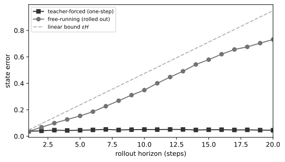
A model is decision-grade for a task not when its predictions look convincing but when using it to choose actions produces reliable decisions under the deployment horizon and feedback rate. The decision, not the reconstruction, is the test. If a planner compares actions by their true returns Q(a) and model returns \hat Q(a), and a^{*} beats the runner-up a^{(2)} by a margin m=Q(a^{*})-Q(a^{(2)}), then the model preserves the winner as long as its return error stays below m/2 everywhere. A large margin tolerates a rough model; a thin margin flips the choice on a tiny error. So we should measure downstream success, not next-frame loss — which is exactly what the planner lets us do.
Receding-horizon control — model-predictive control, the practical cousin of the tree search in Appendix A — limits how long error runs unchecked. At each step, search action sequences under the model, execute only the first (or a short prefix), observe, and replan. Our planner is the simplest such search, random shooting: sample many action sequences, roll each through the model, and keep the one whose imagined trajectory stays closest to the goal (Williams et al. 2017).
# @save
def shooting_plan(model, state, goal, horizon: int, n_samples: int, rng) -> np.ndarray:
    """Pick an action sequence by random-shooting model-predictive control.

    Sample ``n_samples`` random action sequences, roll each through the
    model, and score by *running* distance to the goal (summed over the
    horizon, not just the endpoint) so the first action is a genuine step
    toward the goal. This is the sampling-based MPC used across robotics,
    stripped to its core.

    Args:
        model: A dynamics model with a batched ``step`` method.
        state: Current state, shape ``(2,)``.
        goal: Goal state, shape ``(2,)``.
        horizon: Planning lookahead.
        n_samples: Candidate sequences to sample.
        rng: A NumPy generator.

    Returns:
        The best action sequence, shape ``(horizon, 2)``.
    """
    seqs = rng.uniform(-1, 1, size=(n_samples, horizon, 2)).astype(np.float32)
    states = np.tile(np.asarray(state, np.float32), (n_samples, 1))
    cost = np.zeros(n_samples)
    for t in range(horizon):
        states = model.step(states, seqs[:, t, :])
        cost += np.linalg.norm(states - goal, axis=-1)
    return seqs[int(np.argmin(cost))]


def planning_success(model, horizon: int, replan: bool, n_starts: int = 40,
                     seed: int = 3, budget: int = 30, tol: float = 0.25) -> float:
    """Measure goal-reaching success for open-loop vs receding-horizon control.

    With ``replan=False`` the planner commits the whole ``horizon``-step plan
    before looking again (open loop); with ``replan=True`` it executes one
    step and replans (receding horizon). Everything else is held fixed, so
    the two differ only in how long they trust the model between observations.

    Args:
        model: The dynamics model to plan through.
        horizon: Planning lookahead and open-loop commitment length.
        replan: Whether to replan after every executed step.
        n_starts: Random start/goal pairs to average over.
        seed: Seed for the start/goal sampler.
        budget: Total environment steps allowed per episode.
        tol: Success distance to the goal.

    Returns:
        Fraction of start/goal pairs solved.
    """
    rng = np.random.default_rng(seed)
    starts = rng.uniform(0.5, SIZE - 0.5, size=(n_starts, 2))
    goals = rng.uniform(0.5, SIZE - 0.5, size=(n_starts, 2))
    wins = 0
    for start, goal in zip(starts, goals):
        if np.linalg.norm(start - goal) < 2.0:
            goal = np.clip(goal + 2.5, 0.5, SIZE - 0.5)
        s, steps, commit = start.astype(float), 0, (1 if replan else horizon)
        while steps < budget:
            plan = shooting_plan(model, s, goal, horizon, 256, rng)
            for t in range(commit):
                s = true_step(s, plan[t])
                steps += 1
                if np.linalg.norm(s - goal) <= tol:
                    wins += 1
                    break
                if steps >= budget:
                    break
            else:
                continue
            break
    return round(wins / n_starts, 3)
Now sweep the horizon. For each planning horizon H we run the well-fit model two ways: open-loop, committing the whole H-step plan before observing, and observe-and-replan, executing one step then replanning.
horizons = [1, 2, 4, 8, 12, 16, 20]
open_loop = [planning_success(good, h, replan=False) for h in horizons]
replan = [planning_success(good, h, replan=True) for h in horizons]
print("horizon   ", horizons)
print("open-loop ", open_loop)
print("replan    ", replan)
horizon [1, 2, 4, 8, 12, 16, 20]
open-loop [1.0, 1.0, 0.9, 0.725, 0.6, 0.475, 0.475]
replan [1.0, 1.0, 1.0, 1.0, 0.9, 0.725, 0.575]At short horizons the two agree — with little compounding, planning ahead and replanning are the same. As the horizon grows they separate: open-loop success falls from 1.0 toward 0.48, because the plan is chosen to make the imagined trajectory reach the goal and the real one has drifted away by the end. Observe-and-replan holds far higher through the mid-range — the gap peaks near 0.3 around horizon 12 — because each executed step suffers only one step of model error before a real observation corrects the course. At the very longest horizons even replanning slips, since the planner must still reason through a long, compounding imagined rollout to choose even its first action. Figure 31.6 plots the split.
Show the code that draws this figure
fig, ax = plt.subplots(figsize=(6.2, 3.6))
ax.plot(horizons, open_loop, "o--", color="0.5", label="plan once (open loop)")
ax.plot(horizons, replan, "s-", color="0.15", label="observe and replan")
ax.set(xlabel="planning horizon (steps)", ylabel="goal-reaching success",
       ylim=(0, 1.05))
ax.legend(fontsize=8)
fig.tight_layout()
plt.show()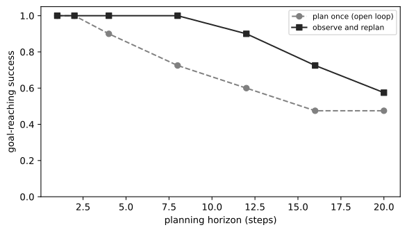
Does replanning simply rescue any model? No — and this is the sharp edge of “decision-grade.” Run the under-fit model, whose one-step error is more than six times larger, with replanning at every step:
print("weak model, replan every step, H=1:", planning_success(weak, 1, replan=True))
print("weak model, replan every step, H=8:", planning_success(weak, 8, replan=True))
weak model, replan every step, H=1: 0.5
weak model, replan every step, H=8: 0.55Even correcting at every single step, the under-fit model reaches the goal only half the time, against the well-fit model’s 1.0. Feedback corrects execution drift; it cannot correct a model that is wrong about the local dynamics in the first place. Impressive one-step numbers, and even frequent feedback, are not substitutes for a model whose errors are small where the decision is made.
NoteIn the interview
Q. A vendor demos a world model with photorealistic rollouts and pitches it for planning warehouse picks. What do you ask for? Not the rollouts — the decisions. Ask for one-step and free-running error over the deployment horizon (the Figure 31.5 split), action-ranking regret and downstream task success under a held-out layout, whether uncertainty rises on interventions absent from training, and the control latency the loop can actually sustain. The trap is grading the video: a model can look flawless and still flip the action at a thin decision margin, and “beautiful rollout” answers none of the five questions decision-grade requires.
Two named failures round this out. Causal confusion is a policy leaning on a correlated cue instead of the cause — braking because brake lights appear in demonstrations, not because the obstacle demands it — and it hides until an intervention breaks the correlation (Haan et al. 2019). Sim-to-real shift is dynamics or appearance differing between training and deployment; domain randomization fights it by varying textures, masses, frictions, and delays during training, a blunt instrument that helps only for the factors it happens to randomize (Tobin et al. 2017). Both are reasons to hold out interventions and shifted scenes, not nearby frames of the same trajectory, when you decide whether a model is decision-grade.
31.7 Simulators, grounded skills, and rare events
Everything we just did — reset to a known state, roll trajectories, grade the outcome — is what a simulator is for. A robotics simulator is not a renderer; it is a controlled environment with reset, step, observation, and privileged-state-query interfaces, and used well it is three instruments at once: a data generator, an evaluation harness, and a rare-event factory. Its defining property is that the grader reads state the policy cannot touch. A policy can announce “done,” emit a fluent explanation, or collect a shaped reward while the object sits outside the target; only privileged state settles it. For N episodes with a versioned final-state predicate G_i, the suite score is
\widehat S=\frac{1}{N}\sum_{i=1}^{N}\mathbf 1\!\left[G_i(s_T)=\text{true}\right], \tag{31.5}
exactly the environment-graded rate our vla_success and planning_success already compute. Figure 31.7 locates where ground truth lives.
flowchart TB
    SPEC["Versioned task spec<br/>goal + initial-state distribution"] -->|configure| SIM[("Simulator state<br/>physics, contacts")]
    RARE["Rare-event sampler<br/>shift parameters"] -->|scenario seed| SIM
    SIM -->|rendered observation| POLICY(["Policy under test"])
    POLICY -->|action| ADAPTER["Action adapter<br/>frame, units, limits"]
    ADAPTER --> SIM
    SIM -->|privileged state| DATA["Training-data generator"]
    SIM -->|final state| GRADER["Deterministic predicate"]
    GRADER --> REPORT[("Report<br/>versions, seeds, latency")]
The rare-event role is why a simulator beats collecting logs: an experiment can over-sample slippery contacts, occlusions, or near-limit states that a fleet might see once a month, then restore deployment weights when reporting the expected product metric. This is the same seam Chapter 23 built its refund gym on and the same digital-twin grading Chapter 22 uses for statistics — a training distribution deliberately unlike production, with a grader that reads state. Fidelity is a budget, not a virtue: detailed contact physics earns its cost for insertion tasks and wastes it for open-floor navigation, so tie every simulator feature to a specific failure it is meant to predict. Simulators such as LIBERO and SimplerEnv for manipulation, and Habitat for navigation, differ in task vocabulary but share this contract (Liu et al. 2023; Li et al. 2024; Szot et al. 2021).
An hour-long task is rarely one monolithic policy. It composes grounded skills — navigate, grasp, open, place — each a closed-loop behavior with preconditions. SayCan makes the composition explicit: a language model scores how well each skill advances the instruction, and an affordance model scores whether the robot can do it now, and the two multiply (Ahn et al. 2022):
k^{*}=\arg\max_k\; p_{\text{lang}}(k\mid g)\;p_{\text{aff}}(\text{success}\mid o,k). \tag{31.6}
The affordance factor is grounding, not prompting, and it is what stops the plan from proposing something sensible-sounding but impossible. A worked example: the instruction is “wipe up the spill.”
# @save
def saycan_select(skills, p_lang, p_aff):
    """Pick a skill by SayCan's language-times-affordance product (@eq-ch31-saycan).

    Args:
        skills: Candidate skill names.
        p_lang: Language relevance of each skill to the instruction.
        p_aff: Grounded probability each skill can succeed right now.

    Returns:
        ``(best_skill, products)``: the winner and the per-skill products.
    """
    products = [l * a for l, a in zip(p_lang, p_aff)]
    return skills[int(np.argmax(products))], products
skills = ["pick up sponge", "wipe table", "pick up mug", "open drawer"]
p_lang = [0.35, 0.45, 0.05, 0.15] # relevance to "wipe up the spill"
p_aff = [0.95, 0.15, 0.90, 0.85] # feasible now (the spill is out of reach)
best, products = saycan_select(skills, p_lang, p_aff)
print("language alone would pick:", skills[int(np.argmax(p_lang))])
print("SayCan picks: ", best)
print("products:", [round(p, 3) for p in products])language alone would pick: wipe table
SayCan picks: pick up sponge
products: [0.332, 0.068, 0.045, 0.128]Language alone would try to wipe immediately — the most relevant verb. Grounding vetoes it, because the spill is out of reach, and the product picks up the sponge first, the feasible step that makes wiping possible. Figure 31.8 shows the flip.
Show the code that draws this figure
import numpy as np
x = np.arange(len(skills))
fig, ax = plt.subplots(figsize=(6.4, 3.2))
ax.bar(x - 0.25, p_lang, 0.25, label="p(language)", color="0.7")
ax.bar(x, p_aff, 0.25, label="p(affordance)", color="0.45")
ax.bar(x + 0.25, products, 0.25, label="product", color="0.15")
ax.set_xticks(x)
ax.set_xticklabels(skills, rotation=15, fontsize=8)
ax.legend(fontsize=8)
fig.tight_layout()
plt.show()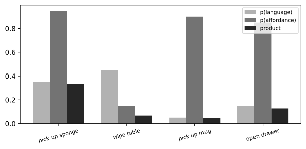
Code as Policies pushes the same idea further, letting the language model write policy code against an allowlisted robot API — expressive, but it crosses a code-execution boundary that needs the sandboxing and approval machinery of Chapter 17. And more robots are not automatically better: multi-agent embodiment adds assignment, collision avoidance, and shared-world consistency, and Chapter 20’s coordination economics decide whether a second robot’s parallel progress beats its interference cost.
31.8 Physical-world safety and open problems
Physical safety starts below the model. Certified controllers, workspace and force limits, watchdogs, and an emergency stop must keep working when inference stalls or emits nonsense; the model supplies intent inside that envelope, it does not replace it. Above that floor sits the one seam this chapter owns: deciding which proposals get physical authority. Chapter 16 built the agent loop as propose → gate → execute, where a gate returns allow-or-deny before any tool runs. The embodied version asks a reversibility question — is this action large or forceful enough that a mistake cannot be undone?
# @save
def reversibility_gate(action, approve=None, max_disp: float = 0.9, max_force: float = 8.0) -> bool:
    """Authorize an action, escalating irreversible ones for confirmation.

    The same propose-gate-execute seam as @sec-ch16, specialized to physical
    consequence: small, low-force actions pass automatically; a large
    displacement or a hard predicted contact force requires an explicit
    approval callback, and with none the action is denied. A real gate reads
    validated force and geometry, not this toy heuristic — but the control
    point is the placement, not the threshold.

    Args:
        action: Proposed action; first coords are displacement, last is grip.
        approve: Callback that returns True to authorize an escalated action.
        max_disp: Displacement magnitude allowed without approval.
        max_force: Predicted contact force (N) allowed without approval.

    Returns:
        True if the action may execute, False if it is held.
    """
    disp = float(np.linalg.norm(action[:2]))
    force = float(max(0.0, -action[-1]) * 12.0)  # a firm grasp implies contact force
    if disp <= max_disp and force <= max_force:
        return True
    return bool(approve and approve({"displacement": disp, "predicted_force_n": force}))
gentle = np.array([0.3, 0.2, 0.0])
lunge = np.array([1.0, 0.9, -1.0]) # large move + hard grasp
print("gentle move ->", reversibility_gate(gentle))
print("lunging grasp, no ok ->", reversibility_gate(lunge))
print("lunging grasp, approved ->", reversibility_gate(lunge, approve=lambda p: True))gentle move -> True
lunging grasp, no ok -> False
lunging grasp, approved -> TrueThe gentle action passes; the lunging grasp is denied until an approver signs off on the exact proposal. Figure 31.9 is the state machine behind those three lines: authority is granted only to fresh, in-envelope actions, and any denial, stale observation, or watchdog event falls to a safe hold.
stateDiagram-v2
    [*] --> Observed
    Observed --> Proposed: policy output + observation id
    Proposed --> Executing: fresh and in-envelope
    Proposed --> AwaitingApproval: escalated action
    Proposed --> SafeHold: stale / invalid / watchdog
    AwaitingApproval --> Executing: approval binds exact proposal
    AwaitingApproval --> SafeHold: deny / timeout / changed state
    Executing --> Observed: new sensor frame
    Executing --> SafeHold: controller fault / e-stop
    SafeHold --> Observed: authorized reset
Approval binds the exact action and the observation identity, because a fresh frame can invalidate an old approval — the world may have moved between review and execution, the time-of-check/time-of-use hazard Chapter 17 owns. And the perception feeding the gate is itself attackable: a texture patch, a projected pattern, or a compromised camera can steer a vision policy, so the gate should consume independently validated state where it can — Chapter 24 owns adversarial perception and policy enforcement. Human approval is one control nested inside hard physical limits, not a substitute for them; a reviewer without depth or contact information cannot make an unsafe trajectory safe.
The open problems are where these threads fray. Data diversity, hardware time, and expensive failure recovery still bound embodied learning; contact-rich and deformable tasks amplify the small state errors Figure 31.5 made visible; evaluation has no universal task set, and a final-state average can hide a catastrophic slice. World models and direct policies may even converge — a policy carries implicit predictive state, a world model can share its representation with a policy — so the label matters less than the evidence. Does the system represent counterfactual consequences, notice when it is outside its envelope, correct with feedback, and reduce real decision regret? Those are the questions our gridworld answered with numbers, and they are the questions a real deployment must answer at scale.
31.9 Summary
We built an embodied agent on a gridworld with a known current, reducing every claim to a printed number. Actions became tokens through a codec bounded by {(K-1)}^{-1}, and a tiny autoregressive policy reached every goal despite imperfect tokens, because the loop was closed. A learned dynamics model predicted one step to within a percent of the box, yet its free-running error compounded past a tenth of the box in twenty steps: open-loop planning collapsed while observe-and-replan held, and feedback did not rescue an under-fit model. Decision-grade is a property of model, planner, horizon, and feedback together — earned by evidence about decisions, not rollouts. Chapter 32 assembles these seams.
31.10 Exercises
Compounding and the Lipschitz bound. Using
rollout_erroron the well-fit model, estimate the empirical growth rate of the free-running error and compare it to the bound in Equation 31.4.- Fit e_H\approx \epsilon\,(L^H-1)/(L-1) to the measured curve and report the implied L. Is it above or below 1, and what feature of
currentexplains the sign? - Raise
AMPfrom 0.40 to 0.60, retrain the model, and show how both the one-step error and the free-running growth change.
- Fit e_H\approx \epsilon\,(L^H-1)/(L-1) to the measured curve and report the implied L. Is it above or below 1, and what feature of
Where open-loop and replan diverge. In
planning_success, sweep the horizon finely and find the horizon at which open-loop success first drops below observe-and-replan by more than 0.2. Relate that horizon to the free-running error at which the drift first exceeds the goal tolerancetol.Is your model decision-grade? Train dynamics models on 40, 200, 1000, and 8000 transitions. For each, plot one-step RMSE on one axis and observe-and-replan planning success (at horizon 8) on the other. Where does one-step error stop predicting planning success, and why is that the whole point of the section?
The action contract. Change
ACTION_BINSto 5 and to 41, retrain the token policy each time, and report closed-loop success and within-1-bin accuracy. Then corrupt the gripper convention by negating the last coordinate before tokenizing and describe the failure — even though every token is valid.A grader you can game. Add an obstacle to the gridworld and a policy that reaches the goal by pushing through it. Write a final-state predicate that still marks the episode successful, then add one trajectory-aware predicate that catches the violation, and state which product requirement justifies its cost (Chapter 22 owns the statistics).
Grounding flips the plan. In the SayCan example, find the affordance value for “wipe table” at which it becomes the selected skill, holding the language scores fixed. Then construct an instruction and scores where language and affordance disagree on every skill, and describe what the robot should do next.
The reversibility envelope. Instrument
reversibility_gateto count how often it escalates during a fullvla_successrun, then tightenmax_dispuntil the escalation rate exceeds 25%.- What does that rate tell you about the policy’s typical action magnitude?
- Design an approval callback that auto-approves near a known-safe region of the box but escalates elsewhere, and argue why binding the approval to the observation id (not just the action) matters when the world is changing.