28  Agent Products, People, and Organizations

We are now ready to compute a launch decision. Chapter 27 keeps a deployed agent running — its SLOs, its incidents, its review queue. This chapter asks a different question about the same agent: should this product exist in this form, for these people, under this organization, at this autonomy level? We answer it by assembling one artifact, the launch-review appendix, out of numbers the chapter computes in front of you: (i) a plan diff and a receipt that make the agent’s state legible; (ii) the reliance matrix that separates appropriate reliance from over- and under-reliance, by cohort; (iii) the invocation-to-outcome funnel, where an offline eval score and realized product value visibly diverge; (iv) cost per outcome under three product designs, with review labor charged honestly; (v) accessibility completion as a gate, not an afterthought; (vi) a NIST-style risk-register entry joined to those gate results; and (vii) the assembled appendix that reads off a recommendation. The running example is a synthetic but deliberately awkward one: an expense-triage agent that is economically attractive and still not ready to launch.

The awkwardness is the lesson. A release argument is three nested claims, and it passes only if all three hold at once. The user claim: a person can form an accurate picture of what the agent is doing and intervene. The product claim: use causes a worthwhile outcome against a simpler baseline. The organization claim: named owners can keep the claim true through change. These do not average. Product value cannot buy back an excluded cohort; a complete policy binder cannot manufacture a useful outcome. Our expense agent will pass the money argument and fail the people argument, and the whole point of computing the evidence is that no single green dashboard can hide that.

One honesty note before we start. Every number on these pages is computed live from a small synthetic cohort log we define in full and can read. It is representative, not a recorded production run — the tension it encodes (new reviewers over-trusting the agent, assistive-technology users abandoning a streaming flow) is one we built on purpose so the decision is reproducible. The mechanisms — the reliance cells, the funnel joins, the cost decomposition, the gate evaluation — are exactly the ones a real launch review runs; only the constants would change.

28.1 Make the agent legible: plan diffs, receipts, and epistemic labels

An agent that acts on the world owes its user two objects before and after every effect, and neither is a sentence of prose. Before an effect, a plan diff: the exact change proposed — which object, which field, from what state to what state, under whose permission — so a person can approve the specific delta rather than a vibe. After an effect, a receipt: the authoritative system, the operation’s identity, the committed result, a timestamp, and whether it reconciled with downstream state. A chat bubble that says “done” is not a receipt; it is the model narrating, and the model’s narration is the one thing in the system we cannot audit. We build both as small typed objects so they are inspectable, testable, and impossible to fake with fluent text.

The evidence a plan diff carries also needs provenance. The same screen may show a fact read from an authoritative system, a value the user typed, an inference the model drew, and a question nobody has answered yet — and collapsing those into one confident paragraph is how overreliance starts. We fix a small vocabulary of epistemic labels and apply it to every claim.

# @save
from __future__ import annotations

from collections import Counter
from dataclasses import dataclass
from enum import Enum


class EpistemicLabel(str, Enum):
    """The provenance a product attaches to each claim it shows a user.

    Distinguishing a sourced fact from a model inference from an unresolved
    question is what lets a reviewer calibrate trust to evidence instead of to
    fluent phrasing. The labels are stable strings so the same word means the
    same thing on every screen and in every modality.
    """

    SOURCE_FACT = "source fact"
    USER_PROVIDED = "user-provided"
    SYSTEM_STATE = "system state"
    MODEL_INFERENCE = "model inference"
    ESTIMATE = "estimate"
    UNRESOLVED = "unresolved"

The plan diff and the receipt are the two halves of one accountable action. We keep them as frozen dataclasses so an approval binds an exact proposal and a receipt records exactly what committed.

# @save
@dataclass(frozen=True)
class PlanDiff:
    """The exact change an agent proposes, shown before any effect runs.

    A person should approve this delta, not a summary of it: the affected
    object and field, the current and proposed state, the permission the
    effect would exercise, and the labeled evidence behind it. Approving a
    plan diff is narrow by construction; approving "the plan" is not.
    """

    affected_object: str
    field: str
    from_state: str
    to_state: str
    permission: str
    evidence: tuple[tuple[EpistemicLabel, str], ...]


@dataclass(frozen=True)
class Receipt:
    """The record of an effect after it commits, tied to authoritative state.

    Unlike a generated "done" message, a receipt names the system of record,
    the operation identity a later reconciliation can join on, the committed
    result, when it happened, and whether downstream state agrees. It is the
    product-level analogue of Chapter 16's effect log.
    """

    system: str
    op_id: str
    result: str
    timestamp: str
    reconciliation: str

Here is one real instance for the expense agent: it proposes writing a category to a specific record, backed by three differently-sourced pieces of evidence, and — once a reviewer approves — the receipt that comes back.

proposal = PlanDiff(
    affected_object="expense EXP-4471",
    field="category",
    from_state="(uncategorized)",
    to_state="Travel",
    permission="write:expense_category",
    evidence=(
        (EpistemicLabel.SOURCE_FACT, "Merchant on receipt is 'Delta Air Lines', amount 48.00 units"),
        (EpistemicLabel.MODEL_INFERENCE, "Airfare under 50 units is most often 'Travel' for this unit"),
        (EpistemicLabel.UNRESOLVED, "Two required itemized receipts are missing"),
    ),
)
print(f"PLAN DIFF  {proposal.affected_object}")
print(f"  {proposal.field}: {proposal.from_state} -> {proposal.to_state}  [{proposal.permission}]")
for label, statement in proposal.evidence:
    print(f"  - ({label.value}) {statement}")

approved = Receipt(
    system="expense-ledger",
    op_id="op-9f2a41",
    result="category=Travel written to EXP-4471",
    timestamp="2026-07-19T14:03:07Z",
    reconciliation="ledger echo confirmed; 2 receipts still pending",
)
print(f"\nRECEIPT    {approved.system}  {approved.op_id}")
print(f"  {approved.result}")
print(f"  at {approved.timestamp}  |  reconciliation: {approved.reconciliation}")

PLAN DIFF  expense EXP-4471
  category: (uncategorized) -> Travel  [write:expense_category]
  - (source fact) Merchant on receipt is 'Delta Air Lines', amount 48.00 units
  - (model inference) Airfare under 50 units is most often 'Travel' for this unit
  - (unresolved) Two required itemized receipts are missing

RECEIPT    expense-ledger  op-9f2a41
  category=Travel written to EXP-4471
  at 2026-07-19T14:03:07Z  |  reconciliation: ledger echo confirmed; 2 receipts still pending

Read the two objects together. The plan diff surfaces the one thing a reviewer must weigh — an inference about category resting on an unresolved evidence gap — instead of burying it under a confident recommendation. The receipt then closes the loop against the ledger, and its reconciliation field refuses to claim more than it can: the write committed, but two receipts are still pending. Figure 28.1 names the anatomy of both.

flowchart TB
    subgraph PD["PLAN DIFF — shown before the effect"]
        A1["affected object + field"]
        A2["from-state → to-state"]
        A3["permission exercised"]
        A4["evidence, each epistemically labeled"]
    end
    PD -->|"reviewer approves this exact delta"| EFF(["effect commits"])
    EFF --> RC
    subgraph RC["RECEIPT — shown after the effect"]
        B1["system of record"]
        B2["operation id (joinable)"]
        B3["result + timestamp"]
        B4["reconciliation status"]
    end

Figure 28.1: What must an agent show around an effect? A plan diff before (labeled delta and evidence) and a receipt after (authoritative record and reconciliation) — neither of which a prose ‘done’ can supply.

Two design rules follow from having built these objects. Initiative should move by expected value: a low-consequence, reversible change may proceed silently, but a novel payee, an uncertain policy reading, or an irreversible submission must surface a plan diff and wait (Horvitz 1999). And personalization is a labeled, resettable object like any other — a remembered preference is inspectable and scoped, a reset removes it from every surface that consumes it, and no sensitive preference is ever inferred merely because it predicts clicks. The guidelines literature validated across a product lifecycle says the same in aggregate (Amershi et al. 2019); here it is two dataclasses and a rule about when to show them.

28.2 Measure appropriate reliance, not engagement

Trust is an attitude; reliance is a behavior we can count — accepting, rejecting, checking, overriding. A product that optimizes “trust” as a scalar invites manipulation, so we optimize the thing we can observe and ground: reliance that tracks the agent’s actual capability (Lee and See 2004). That means separating four outcomes, not one. For a set of recommendations whose correctness is established downstream, each reviewer decision falls into exactly one cell of a two-by-two: the recommendation was correct or wrong, and the person accepted or rejected it.

R_\text{app}=\frac{N_{CA}+N_{WR}}{N},\qquad R_\text{over}=\frac{N_{WA}}{N_{WA}+N_{WR}},\qquad R_\text{under}=\frac{N_{CR}}{N_{CA}+N_{CR}}, \tag{28.1}

where N_{CA} is correct-accept, N_{WR} wrong-reject, N_{WA} wrong-accept, N_{CR} correct-reject, and N the total. Appropriate reliance rewards two behaviors at once: accepting good help and catching bad help. Overreliance is the share of the agent’s wrong recommendations a person waves through; underreliance is the share of its good recommendations a person needlessly discards. A single “agreement with AI” number blends the harmless N_{CA} with the dangerous N_{WA} and hides both failure modes. So does engagement: acceptance, daily use, and satisfaction can all climb while judgment rots.

We need the raw material. Our synthetic cohort log holds three groups with a deliberate structure — experienced reviewers who catch most bad recommendations, new reviewers who accept almost anything, and assistive-technology users who struggle to finish at all. Each cohort carries its four reliance counts, how many rejections were confirmed to have caught a real defect, its average review time, and a nested usage funnel we return to later.

# @save
QUADRANTS = ("correct_accept", "correct_reject", "wrong_accept", "wrong_reject")
STAGES = ("exposed", "invoked", "completed", "accepted_or_edited", "outcome_realized", "retained")

COHORT_LOG = {
    "experienced": {
        "size": 200,
        "quadrants": {"correct_accept": 160, "correct_reject": 10, "wrong_accept": 4, "wrong_reject": 26},
        "confirmed_catches": 24, "review_seconds": 35,
        "funnel": {"exposed": 200, "invoked": 190, "completed": 180,
                   "accepted_or_edited": 170, "outcome_realized": 160, "retained": 145},
    },
    "new_reviewer": {
        "size": 200,
        "quadrants": {"correct_accept": 165, "correct_reject": 5, "wrong_accept": 25, "wrong_reject": 5},
        "confirmed_catches": 5, "review_seconds": 85,
        "funnel": {"exposed": 200, "invoked": 185, "completed": 175,
                   "accepted_or_edited": 155, "outcome_realized": 140, "retained": 115},
    },
    "assistive_technology": {
        "size": 100,
        "quadrants": {"correct_accept": 70, "correct_reject": 10, "wrong_accept": 5, "wrong_reject": 15},
        "confirmed_catches": 14, "review_seconds": 70,
        "funnel": {"exposed": 100, "invoked": 85, "completed": 65,
                   "accepted_or_edited": 55, "outcome_realized": 45, "retained": 35},
    },
}

The compact counts expand into a per-decision ledger — one row per reviewed case — so every later metric is a slice-and-count over the same 500 rows rather than a headline we have to trust. A parallel usage ledger records, per exposed case, how far it advanced through the funnel.

# @save
def expand_logs(cohorts: dict) -> tuple[list[dict], list[dict]]:
    """Expand compact cohort counts into two aligned per-case ledgers.

    The reviewer-decision ledger has one row per reviewed case tagged with its
    reliance quadrant and whether its rejection was a confirmed catch; the
    usage ledger has one row per exposed case flagged with the funnel stages it
    reached. Working from per-case rows means every reported rate is a count
    over a slice, which is what makes cohort breakdowns honest.

    Args:
        cohorts: The cohort log mapping each group to its counts and funnel.

    Returns:
        A tuple ``(decisions, usage)`` of two row lists.
    """
    decisions: list[dict] = []
    usage: list[dict] = []
    case_id = 0
    for name, cohort in cohorts.items():
        for quadrant in QUADRANTS:
            for offset in range(cohort["quadrants"][quadrant]):
                decisions.append({
                    "case_id": case_id, "cohort": name, "quadrant": quadrant,
                    "confirmed_catch": quadrant == "wrong_reject" and offset < cohort["confirmed_catches"],
                    "review_seconds": cohort["review_seconds"],
                })
                case_id += 1
        for index in range(cohort["size"]):
            usage.append({"cohort": name, **{stage: index < cohort["funnel"][stage] for stage in STAGES}})
    return decisions, usage


decisions, usage = expand_logs(COHORT_LOG)
print(f"reviewer decisions: {len(decisions)}   usage rows: {len(usage)}")
print("one decision row:", decisions[0])

reviewer decisions: 500   usage rows: 500
one decision row: {'case_id': 0, 'cohort': 'experienced', 'quadrant': 'correct_accept', 'confirmed_catch': False, 'review_seconds': 35}

Now the metric of Equation 28.1, computed over any slice of decision rows. Keeping all four cells intact — rather than reducing to one agreement number too early — is the entire discipline.

# @save
def reliance_rates(rows) -> dict:
    """Compute the four-cell reliance rates for one slice of decisions.

    Returns appropriate reliance (correct-accept plus wrong-reject over all),
    overreliance (accepting the agent's wrong recommendations), and
    underreliance (rejecting its good ones), plus a confirmed-catch rate that
    asks whether a rejection prevented a real defect or merely made rework.
    Reporting all of these keeps a harmless correct-accept from masking a
    dangerous wrong-accept.

    Args:
        rows: An iterable of decision rows, each carrying a ``quadrant`` key.

    Returns:
        A dict of counts and the rates from @eq-ch28-reliance.
    """
    rows = list(rows)
    counts = Counter(row["quadrant"] for row in rows)
    correct = counts["correct_accept"] + counts["correct_reject"]
    wrong = counts["wrong_accept"] + counts["wrong_reject"]
    catches = sum(row["confirmed_catch"] for row in rows)
    return {
        "n": len(rows),
        "quadrants": {name: counts[name] for name in QUADRANTS},
        "appropriate_rate": round((counts["correct_accept"] + counts["wrong_reject"]) / len(rows), 4),
        "overreliance_rate": round(counts["wrong_accept"] / wrong, 4),
        "underreliance_rate": round(counts["correct_reject"] / correct, 4),
        "confirmed_catch_rate": round(catches / counts["wrong_reject"], 4),
    }


def reliance_report(decisions: list[dict]) -> dict:
    """Compute overall reliance and one breakdown per cohort.

    Args:
        decisions: The reviewer-decision ledger from ``expand_logs``.

    Returns:
        A dict with ``overall`` rates and a ``by_cohort`` mapping.
    """
    cohorts = sorted({row["cohort"] for row in decisions})
    return {
        "overall": reliance_rates(decisions),
        "by_cohort": {name: reliance_rates(r for r in decisions if r["cohort"] == name) for name in cohorts},
    }


reliance = reliance_report(decisions)
overall = reliance["overall"]
print(f"overall appropriate={overall['appropriate_rate']}  "
      f"over={overall['overreliance_rate']}  under={overall['underreliance_rate']}")

overall appropriate=0.882  over=0.425  under=0.0595

The aggregate looks almost launch-ready: an appropriate rate of 0.882, with most disagreement being harmless. The reliance matrix makes the four cells concrete — and labels which cell means what.

import matplotlib.pyplot as plt
import numpy as np
from matplotlib_inline.backend_inline import set_matplotlib_formats

plt.rcParams["svg.hashsalt"] = "chapter-28"
set_matplotlib_formats("svg", metadata={"Date": None})

q = overall["quadrants"]
values = np.array([[q["correct_accept"], q["correct_reject"]],
                   [q["wrong_accept"], q["wrong_reject"]]])
labels = np.array([["appropriate", "underreliance"], ["overreliance", "appropriate"]])
fig, ax = plt.subplots(figsize=(6.6, 3.4))
ax.imshow(values, cmap="Blues", vmin=0, vmax=values.max())
ax.set_xticks([0, 1], ["Accept", "Reject"])
ax.set_yticks([0, 1], ["Correct", "Wrong"])
ax.set_xlabel("Reviewer decision")
ax.set_ylabel("Recommendation correctness")
for r in range(2):
    for c in range(2):
        shade = "white" if values[r, c] > values.max() / 2 else "black"
        ax.text(c, r, f"{values[r, c]}\n{labels[r, c]}", ha="center", va="center",
                color=shade, fontweight="bold")
ax.set_title("Reviewer decisions (n = 500)")
fig.tight_layout()
plt.show()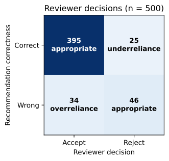

Figure 28.2: Where does the whole reviewer population rely appropriately, and where not? The diagonal (correct-accept, wrong-reject) is appropriate reliance; the off-diagonal splits into overreliance (accept a wrong recommendation) and underreliance (reject a correct one).

Now the reason the aggregate lies. Averaging blends the population that already exists (experienced reviewers) with the population a rollout creates (new reviewers), and those behave nothing alike. We plot overreliance per cohort against the overall number.

by_cohort = reliance["by_cohort"]
names = ["experienced", "assistive_technology", "new_reviewer"]
over = [by_cohort[n]["overreliance_rate"] for n in names]
fig, ax = plt.subplots(figsize=(6.6, 3.4))
bars = ax.bar(names, over, color=["#2a7f9e", "#b7791f", "#b13f3f"], width=0.6)
ax.axhline(0.25, ls="--", color="0.4")
ax.text(2.35, 0.28, "cohort gate 0.25", fontsize=8, ha="right", color="0.3")
ax.axhline(overall["overreliance_rate"], ls=":", color="0.55")
ax.text(0.0, overall["overreliance_rate"] + 0.02, f"overall {overall['overreliance_rate']}", fontsize=8, color="0.4")
for bar, value in zip(bars, over):
    ax.text(bar.get_x() + bar.get_width() / 2, value + 0.02, f"{value}", ha="center", fontsize=9)
ax.set_ylabel("overreliance rate")
ax.set_ylim(0, 1)
fig.tight_layout()
plt.show()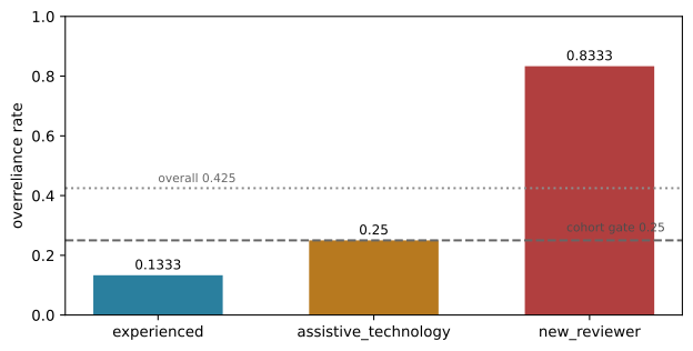

Figure 28.3: Why does an aggregate appropriate rate of 0.882 hide a cohort in trouble? Overreliance is near zero for experienced reviewers but 0.833 for new reviewers — the population a rollout manufactures — far above the 0.25 gate.

The new-reviewer bar is the chapter in one figure: 25 of their 30 wrong recommendations were accepted, an overreliance rate of 0.833, more than three times the gate. Their confirmed-catch rate tells the same story from the other side — they almost never reject anything. An interface that shows the evidence and the exact proposed write before the recommendation, or that asks for an initial judgment on high-uncertainty cases, can move these cells; a confidence badge shown on every case becomes wallpaper and can anchor a poorly-calibrated user (Buçinca et al. 2021). The right way to know is to test each intervention on all four cells plus decision time and accessibility — not on satisfaction in isolation.

NoteIn the interview

Q. Your assistant’s acceptance rate and daily-active use are both up 20% after a launch. Is that good? It is not evidence of anything good on its own. Acceptance and engagement rise when overreliance rises — a new cohort that waves everything through looks identical to a delighted one on those metrics. The answer they want: measure appropriate reliance against outcome-grounded correctness, split by cohort, and check overreliance and underreliance separately; a rise in acceptance with a rise in wrong-accepts is a regression, not a win. The trap is treating engagement as the goal metric, or reporting one aggregate agreement number.

28.3 Make accessibility a correctness property

Accessibility is not a compliance pass bolted on after model quality. For an agent it is a control property: a person who cannot perceive a plan cannot supervise it, and a person who cannot operate the approve control cannot stop an effect. So we measure the same funnel by access mode and gate it, exactly as we gate reliance. Our assistive-technology cohort exposes the failure: 85 of them invoke the agent, but only 65 finish the recommendation step, because the streaming review flow moves focus on every token and never announces a stable completion state.

at = COHORT_LOG["assistive_technology"]["funnel"]
completion = round(at["completed"] / at["invoked"], 4)
floor = 0.85
print(f"assistive invoked -> completed: {at['completed']}/{at['invoked']} = {completion}  (floor {floor})")
print("passes accessibility gate:", completion >= floor)

assistive invoked -> completed: 65/85 = 0.7647  (floor 0.85)
passes accessibility gate: False

A completion of 0.765 against a 0.85 floor is not a rounding error to ship past; it is one in five users of a supported access mode excluded from finishing a task their colleagues finish. The engineering response is to diagnose the interaction and repair it — here, a non-streaming fallback that announces completion instead of flooding a live region — and then re-measure, never to lower the gate after seeing the result. Suppose the repair recovers the users who abandoned specifically at the streaming step. We can project the effect honestly and check whether it would clear the gate.

recovered = 9  # representative: users who abandoned at the streaming step, not a measured result
repaired_completed = at["completed"] + recovered
repaired = round(repaired_completed / at["invoked"], 4)
print(f"projected after non-streaming fallback: {repaired_completed}/{at['invoked']} = {repaired}")
print("would clear the 0.85 floor:", repaired >= floor)

projected after non-streaming fallback: 74/85 = 0.8706
would clear the 0.85 floor: True

Plotting the measured flow against the projected repair puts the gate decision in one frame: one bar sits below the floor, the other just above it.

fig, ax = plt.subplots(figsize=(5.6, 3.2))
bars = ax.bar(["streaming\n(measured)", "non-streaming\n(projected)"], [completion, repaired],
              color=["#b13f3f", "#2a7f9e"], width=0.55)
ax.axhline(floor, ls="--", color="0.4")
ax.text(1.42, floor + 0.008, "floor 0.85", fontsize=8, ha="right", color="0.3")
for bar, value in zip(bars, [completion, repaired]):
    ax.text(bar.get_x() + bar.get_width() / 2, value + 0.01, f"{value}", ha="center", fontsize=9)
ax.set_ylabel("invoked → completed")
ax.set_ylim(0, 1)
fig.tight_layout()
plt.show()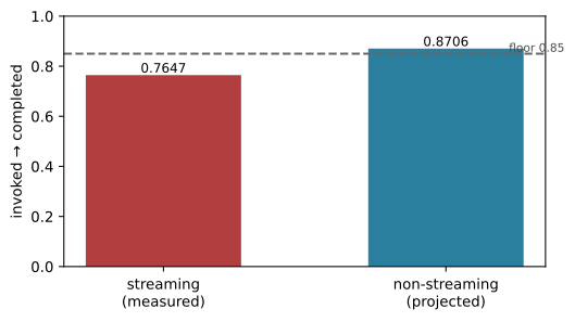

Figure 28.4: Does the accessibility gate change the decision? The streaming flow completes 0.765 of assistive-technology invocations, below the 0.85 floor; a projected non-streaming fallback that recovers nine abandoned users would clear it — evidence to gather, not assume.

The projection is labeled a projection: it tells us the repair is worth building and re-testing with real assistive-technology users, not that the cohort now passes. Accessibility ownership also has to survive procurement — a vendor’s conformance report is evidence about a named version and scope, not a transferable guarantee for your prompts, generated content, wrapper, and tools; the product team still owns end-to-end task testing in its own scaffold. And the same seriousness extends to language and locale: a fluent response is not necessarily an accurate or culturally suitable action, so the end-to-end task is evaluated with people who use the language in context.

28.4 Discover value before autonomy; declare kill criteria

Before pricing the agent we ask whether it should be an agent at all. Agents earn their complexity when the path to an outcome is variable, information-rich, and partly judgmental — the same properties that make them expensive to run and hard to evaluate. So we begin with the least agentic design that could produce the value and make it earn every added rung. For the expense task there are three candidates: a deterministic rules workflow that auto-settles the safe subset, a single-call classifier that labels every case, and the bounded agent we have been measuring. We price all three on the same denominator: cost per realized outcome, with review labor — the work the product shifts onto humans — charged in full.

# @save
REVIEW_HOURLY_RATE = 36.0
BASELINE_COST_PER_OUTCOME = 1.60

DESIGNS = {
    "deterministic_rules": {"machine": 5.0, "review_seconds": 6000, "remediation": 0.0, "outcomes": 250},
    "single_call_classifier": {"machine": 20.0, "review_seconds": 22500, "remediation": 48.0, "outcomes": 300},
    "bounded_agent": {"machine": 45.0, "review_seconds": 31000, "remediation": 136.0, "outcomes": 345},
}


def cost_per_outcome(machine: float, review_seconds: float, remediation: float,
                     outcomes: int, rate: float = REVIEW_HOURLY_RATE) -> dict:
    """Price one design's realized outcomes, review labor charged in full.

    The denominator is a realized, quality-qualified outcome — not an
    invocation or a token. Review labor (reading, checking, correcting) is the
    hidden cost a product shifts onto humans, so it enters the numerator at the
    reviewer's hourly rate rather than being waved away as "free" human time.

    Args:
        machine: Inference and retrieval cost for the window.
        review_seconds: Total human review time over all cases.
        remediation: Cost of cleaning up wrong recommendations that slipped through.
        outcomes: Count of realized, quality-qualified outcomes.
        rate: Reviewer cost per hour.

    Returns:
        A dict of the cost components, the total, and the cost per outcome.
    """
    review = review_seconds * rate / 3600.0
    total = machine + review + remediation
    return {
        "machine": round(machine, 2), "review_labor": round(review, 2),
        "remediation": round(remediation, 2), "total_cost": round(total, 2),
        "outcomes": outcomes, "cost_per_outcome": round(total / outcomes, 4),
    }


for name, design in DESIGNS.items():
    row = cost_per_outcome(**design)
    print(f"{name:24} outcomes={row['outcomes']:4}  review={row['review_labor']:6}  "
          f"total={row['total_cost']:6}  per_outcome={row['cost_per_outcome']}")

deterministic_rules      outcomes= 250  review=  60.0  total=  65.0  per_outcome=0.26
single_call_classifier   outcomes= 300  review= 225.0  total= 293.0  per_outcome=0.9767
bounded_agent            outcomes= 345  review= 310.0  total= 491.0  per_outcome=1.4232

The printed rates already surprise; stacking each design’s cost components shows where the money goes, and it is not the machine.

rows = {name: cost_per_outcome(**d) for name, d in DESIGNS.items()}
order = ["deterministic_rules", "single_call_classifier", "bounded_agent"]
short = ["rules", "classifier", "agent"]
machine = [rows[n]["machine"] / rows[n]["outcomes"] for n in order]
review = [rows[n]["review_labor"] / rows[n]["outcomes"] for n in order]
remed = [rows[n]["remediation"] / rows[n]["outcomes"] for n in order]
fig, ax = plt.subplots(figsize=(6.4, 3.6))
ax.bar(short, machine, label="machine", color="#557a3c")
ax.bar(short, review, bottom=machine, label="review labor", color="#b7791f")
ax.bar(short, remed, bottom=[m + r for m, r in zip(machine, review)], label="remediation", color="#b13f3f")
ax.axhline(BASELINE_COST_PER_OUTCOME, ls="--", color="0.4")
ax.text(2.4, BASELINE_COST_PER_OUTCOME + 0.03, "conventional baseline 1.60", fontsize=8, ha="right", color="0.3")
for i, n in enumerate(order):
    ax.text(i, rows[n]["cost_per_outcome"] + 0.03, f"{rows[n]['cost_per_outcome']}", ha="center", fontsize=9)
ax.set_ylabel("cost per realized outcome")
ax.legend(fontsize=8)
fig.tight_layout()
plt.show()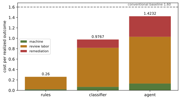

Figure 28.5: Does more autonomy lower cost per outcome? No — the bounded agent has the highest cost per realized outcome (1.42) despite the most outcomes, because review labor grows faster than coverage. All three beat the 1.60 conventional baseline; the question is what the agent’s extra outcomes are worth.

The comparison rewrites the naive story. All three designs beat the 1.60 conventional baseline, so “the agent is cheaper than doing it by hand” is true and almost meaningless. The agent is the most expensive of the three per outcome, at 1.42, because each rung of autonomy grew review labor faster than it grew coverage — the classifier and the agent are dominated by the yellow review band, not by machine cost. The rules workflow settles 250 cases at 0.26 each. The honest question is therefore marginal: the agent’s extra outcomes over the classifier cost (491-293)/(345-300)=4.40 units apiece, far above the baseline. Autonomy has to earn that, and the way we hold it to account is to declare kill criteria before the pilot: appropriate reliance below 0.90, any adequately-sampled cohort over 0.25 overreliance, assistive completion below 0.85, or cost per outcome above the conventional baseline. A threshold chosen after seeing the result is an explanation, not a gate. These four become the code that decides the launch.

28.5 Follow the invocation-to-outcome funnel

A product dashboard usually starts at invocation, because that is where the agent emits its first event. The causal story starts earlier and ends later, and the gap between them is where value leaks. We define a nested funnel — exposed, invoked, completed, accepted-or-edited, outcome-realized, retained — and count each stage as a strict subset of the one before, so a monotone drop is guaranteed and any increase is a bug.

# @save
def _funnel_slice(rows) -> dict:
    """Count the nested funnel stages and adjacent conversions for one slice."""
    rows = list(rows)
    counts = {stage: sum(row[stage] for row in rows) for stage in STAGES}
    conversions = {STAGES[0]: 1.0}
    for prior, stage in zip(STAGES, STAGES[1:]):
        conversions[stage] = round(counts[stage] / counts[prior], 4)
    return {"counts": counts, "conversion_from_previous": conversions}


def funnel_report(usage: list[dict]) -> dict:
    """Compute the invocation-to-outcome funnel overall and per cohort.

    Each stage is a subset of the previous one, so counts never increase and
    the end-to-end rate (outcome-realized over exposed) is the product of the
    adjacent conversions. Keeping both the adjacent and end-to-end views is
    what reveals that a better model-completion step can coexist with falling
    realized value if a later stage — review, integration, downstream
    settlement — quietly worsens.

    Args:
        usage: The usage ledger from ``expand_logs``.

    Returns:
        A dict with ``overall`` and ``by_cohort`` funnel slices.
    """
    cohorts = sorted({row["cohort"] for row in usage})
    return {
        "overall": _funnel_slice(usage),
        "by_cohort": {name: _funnel_slice(r for r in usage if r["cohort"] == name) for name in cohorts},
    }


funnel = funnel_report(usage)
counts = funnel["overall"]["counts"]
end_to_end = round(counts["outcome_realized"] / counts["exposed"], 4)
offline_eval = 0.90  # representative held-out benchmark completion quality
print("funnel:", counts)
print(f"offline eval score={offline_eval}   realized end-to-end value={end_to_end}   gap={round(offline_eval-end_to_end,4)}")

funnel: {'exposed': 500, 'invoked': 460, 'completed': 420, 'accepted_or_edited': 380, 'outcome_realized': 345, 'retained': 295}
offline eval score=0.9   realized end-to-end value=0.69   gap=0.21

Here is the divergence the chapter’s title problem turns on. On a held-out benchmark the agent scores 0.90 — a good model. Followed all the way to a settled reimbursement, it realizes value on 345 of 500 exposed cases: an end-to-end rate of 0.69. The 0.21 gap is not model error; it is invocation reluctance, review friction, integration loss, and abandonment stacked on top of a competent model. Offline evaluation from Chapter 22 remains necessary — it establishes task quality, slice performance, and judge validity — but it cannot see this gap, because it never leaves the model.

stage_names = list(counts.keys())
stage_values = list(counts.values())
fig, ax = plt.subplots(figsize=(6.8, 3.6))
ax.barh(range(len(stage_names)), stage_values, color="#2a7f9e")
ax.set_yticks(range(len(stage_names)), [s.replace("_", " ") for s in stage_names])
ax.invert_yaxis()
for i, v in enumerate(stage_values):
    ax.text(v + 6, i, str(v), va="center", fontsize=9)
ax.axvline(offline_eval * counts["exposed"], ls="--", color="0.35")
ax.text(offline_eval * counts["exposed"], -0.7, "offline eval 0.90", fontsize=8, ha="center", color="0.3")
ax.axvline(end_to_end * counts["exposed"], ls=":", color="0.55")
ax.text(end_to_end * counts["exposed"], 5.7, "realized 0.69", fontsize=8, ha="center", color="0.4")
ax.set_xlabel("cases")
fig.tight_layout()
plt.show()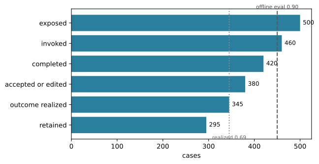

Figure 28.6: Where does the pilot lose people between exposure and value? Each stage drops from the last; the realized end-to-end rate (0.69) sits far below the offline eval score (0.90). The assistive-technology slice loses its largest share exactly at the completion step.

Figure 28.6 forbids the inference that 460 invocations equal 460 outcomes. Every stage needs its own event definition, identity join, and source of truth: a generated answer is completion, not a settled case; a proposed category is not a reimbursement. Two loss patterns deserve instrumentation. Review labor is a hidden funnel stage — reading, evidence retrieval, correction, escalation — and we already charged it in the economics; if almost every case receives a costly approval, a deterministic policy for the safe subset may beat the whole design. And selection into invocation is itself a metric: when the hardest cases avoid the tool, high success among invoked cases can be true and irrelevant, and when only novices invoke it the same aggregate can hide a dependence risk. The controlled-experiment discipline — predeclare the primary outcome, the assignment unit, the stopping rule, and the novelty window — is what keeps a launch dashboard from manufacturing significance (Kohavi et al. 2009).

28.6 Price outcomes, labor, and energy

We have the agent’s cost per outcome from the design comparison; now we assemble it from the ledgers directly, add the break-even review time, and state an energy number with an explicit boundary. Return on investment is always against a counterfactual — the conventional workflow at 1.60 per outcome, not zero — and the denominator is a realized, quality-qualified outcome, with failed and abandoned attempts charged to the population that produced them.

# @save
def economics_report(cohorts: dict, decisions: list[dict], usage: list[dict]) -> dict:
    """Assemble the bounded agent's unit economics from the ledgers.

    Computes cost per realized outcome (machine, review labor, and remediation
    over realized outcomes) and the break-even average review time — the
    longest average review compatible with the conventional baseline — so a
    team can see how interface changes or harder cohorts move the economics.
    Energy is reported per outcome within one stated boundary, useful for
    regression within that boundary and not comparable across different ones.

    Args:
        cohorts: The cohort log (for the energy per-exposure constant).
        decisions: The reviewer-decision ledger.
        usage: The usage ledger.

    Returns:
        A dict of cost components, cost per outcome, break-even seconds, and energy.
    """
    outcomes = sum(row["outcome_realized"] for row in usage)
    review_seconds = sum(row["review_seconds"] for row in decisions)
    wrong_accepts = sum(row["quadrant"] == "wrong_accept" for row in decisions)
    machine = round(len(usage) * 0.09, 2)
    base = cost_per_outcome(machine, review_seconds, wrong_accepts * 4.0, outcomes)
    non_review = base["machine"] + base["remediation"]
    t_max = (BASELINE_COST_PER_OUTCOME * outcomes - non_review) * 3600.0 / (REVIEW_HOURLY_RATE * len(decisions))
    base.update({
        "baseline_cost_per_outcome": BASELINE_COST_PER_OUTCOME,
        "average_review_seconds": round(review_seconds / len(decisions), 1),
        "break_even_review_seconds": round(t_max, 1),
        "energy_wh_per_outcome": round(len(usage) * 0.18 / outcomes, 4),
        "energy_boundary": "representative allocated serving energy; excludes user devices",
    })
    return base


economics = economics_report(COHORT_LOG, decisions, usage)
print(f"cost/outcome={economics['cost_per_outcome']} (baseline {economics['baseline_cost_per_outcome']})  "
      f"avg review={economics['average_review_seconds']}s  break-even={economics['break_even_review_seconds']}s")
print(f"energy={economics['energy_wh_per_outcome']} Wh/outcome  ({economics['energy_boundary']})")

cost/outcome=1.4232 (baseline 1.6)  avg review=62.0s  break-even=74.2s
energy=0.2609 Wh/outcome  (representative allocated serving energy; excludes user devices)

The break-even threshold — 74.2 seconds against an actual average of 62.0 — is a diagnostic, not a target to rush people toward: shorter decisions can raise wrong-accepts, so review time is only ever read alongside reliance. The waterfall shows where the 491 units go and how much slack the review budget has.

comp = [economics["machine"], economics["review_labor"], economics["remediation"]]
comp_names = ["machine", "review\nlabor", "remediation"]
fig, ax = plt.subplots(figsize=(6.4, 3.6))
bottom = 0.0
for value, name, color in zip(comp, comp_names, ["#557a3c", "#b7791f", "#b13f3f"]):
    ax.bar(name, value, bottom=bottom, color=color)
    ax.text(name, bottom + value / 2, f"{value:.0f}", ha="center", va="center", color="white", fontweight="bold")
    bottom += value
ax.bar("total", economics["total_cost"], color="#2a7f9e")
ax.text("total", economics["total_cost"] + 8, f"{economics['total_cost']:.0f}\n= {economics['cost_per_outcome']}/outcome",
        ha="center", fontsize=8)
ax.set_ylabel("cost units")
fig.tight_layout()
plt.show()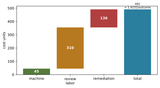

Figure 28.7: How does cost per outcome decompose, and where is break-even? Machine and remediation are small; review labor is the bulk. At 345 outcomes the total (491) divided out is 1.42, under the 1.60 baseline — with review headroom up to a 74.2s average.

Two honest qualifications close the economics. Outcome-based commercial pricing aligns a vendor with a customer only when “outcome” is attributable, quality-qualified, deduplicated, reversible when later invalidated, and protected against gaming — a vendor should not be paid for deflecting a case that returns unresolved. And the energy number carries a question mark by design: 0.26 watt-hours per outcome is meaningful only inside the stated boundary (allocated serving energy, excluding user devices), so it works for regression tests within that boundary and not as a comparison against a differently-scoped published figure (Patterson et al. 2025). The highest-leverage energy optimization is usually product-level — avoid valueless invocations, use the smallest sufficient design — not shortening one prompt. Professional duty runs underneath all of it: disclose material limitations and affected populations, and refuse a launch narrative that relabels a failing slice as “edge cases” without analysis (Association for Computing Machinery 2018).

28.7 Organize for staged autonomy

An agent product crosses application, model, data, platform, security, risk, accessibility, and legal boundaries, and a committee of all of them owns nothing. The durable pattern is a single stream-aligned product team with end-to-end responsibility for the user job, its outcome, its evaluation, and its release, riding a paved road from a platform team — gateway, model catalog, identity, policy enforcement, evaluation infrastructure, tracing, and release evidence — with enabling specialists who transfer capability rather than becoming permanent ticket queues (Skelton and Pais 2019). Centralize what must be consistent (identity, effect policy, required evidence fields); keep judgment near the work (the semantic cost of a wrong category is a product decision, not a platform one). Build-versus-buy is the same allocation in miniature: for every purchased layer you can outsource operation but not accountability, so the contract must pin evaluation access, change notice, accessibility evidence, incident duties, and an exit path — a vendor conformance report is evidence about a version, not a transferable guarantee.

Authority is then granted in rungs, and the rung is set per transition, not per system. Figure 28.8 is the ladder our expense agent is climbing — and where it currently sits.

flowchart TB
    R5["broader autonomy — larger scope, independent oversight<br/><i>advance:</i> sustained evidence across cohorts · <i>revert:</i> any gate outside residual risk"]
    R4["bounded autonomy — allowlisted low-consequence effects<br/><i>advance:</i> outcome SLO, invariant controls · <i>revert:</i> drift or invariant breach"]
    R3["act with approval — proposed effect, human authorization — EXPENSE AGENT is here<br/><i>advance:</i> reviewer discrimination, stable economics · <i>revert:</i> rubber-stamping, review debt"]
    R2["advise — read-only recommendation<br/><i>advance:</i> comprehension, accessibility, reliance lift · <i>revert:</i> failing slice"]
    R1["observe — offline replay, no user effect<br/><i>advance:</i> representative task value · <i>revert:</i> corpus no longer representative"]
    R1 --> R2 --> R3 --> R4 --> R5

Figure 28.8: What advances an agent up the autonomy ladder, and what reverts it? Each rung names the evidence to climb and the condition that sends it back down. Our expense agent is stuck at act-with-approval: the reliance and accessibility evidence for the next rung is failing.

Advancement is not a maturity badge, and reversion must be technically cheap and organizationally legitimate. Three costs accrue at these rungs and belong on the leadership dashboard even though they resist a single metric. Review debt — decisions awaiting independent challenge, expiring exceptions, controls without owners, launch conditions temporarily waived — accrues interest like technical debt; give every item a principal, an owner, a due date, and a repayment test, and never let “risk accepted” become an immortal status. Deskilling — heavy assistance narrows reviewers’ situational awareness until fallback is impossible — is countered by rotating unassisted work and rehearsing degraded modes. And reviewer wellbeing — workload, interruption, exposure to harmful content, and whether incentives reward careful dissent over approval volume — is an organizational property Chapter 27’s queue metrics measure but do not own. The maturity of an agent program is not which rung it reached; it is whether it can descend a rung on evidence without a crisis.

28.8 Operate the AIMS loop

Everything so far is evidence; an AI management system (AIMS) is the repeatable machinery that turns evidence into an accountable decision and keeps it accountable through change. It is not a document folder and not a one-time launch council. The NIST AI Risk Management Framework gives the risk lifecycle four functions: Govern sets culture, roles, and accountability across Map (context, purpose, affected people, impacts), Measure (select and interpret evidence), and Manage (treat risk, accept bounded residual risk through authorized roles, monitor the decision) (National Institute of Standards and Technology 2023). Wrapped around that is the plan-do-check-act cycle of a certifiable management system: plan policy and controls, do the controlled operation, check performance and complaints and control effectiveness, act on nonconformities and changed context (ISO/IEC 2023). Figure 28.9 draws the loop every material change must re-enter.

flowchart LR
    subgraph G["GOVERN — policy · roles · accountability"]
        I["inventory +<br/>immutable bundle"] --> M["MAP<br/>purpose · people · impact"]
        M --> E["MEASURE<br/>reliance · access · funnel · cost"]
        E --> R["MANAGE<br/>treat risk · owner · residual"]
        R --> L{"launch review"}
        L -->|"conditions pass"| O["operate at approved rung"]
        L -->|"hold / constrain / retire"| C["repair or reduce scope"]
        C --> I
        O --> S["outcomes · complaints<br/>incidents · workforce"]
        S -->|"monitoring"| E
        S -->|"material change"| I
    end

Figure 28.9: How does every material product change return through risk evidence and a launch decision? Inventory and context feed measurement and risk treatment into a launch review; operation produces signals; material changes and periodic review loop back — all inside a governing boundary.

The function that makes this concrete is the risk register: each hazard tracked from control to evidence to gate to residual owner. This is where Chapter 25’s governed safety claims become an operating object, because the register’s evidence column is not a promise — it is the metric we just computed, and its status is decided by the gate result. First the gate evaluation the register joins against.

# @save
KILL_CRITERIA = {"minimum_appropriate_rate": 0.90, "maximum_cohort_overreliance": 0.25,
                 "minimum_assistive_completion": 0.85}


def evaluate_gates(reliance: dict, funnel: dict, economics: dict, kill: dict = KILL_CRITERIA) -> list[dict]:
    """Evaluate the four predeclared launch gates against computed evidence.

    The gates are conjunctive: reliance, cohort overreliance, accessibility
    completion, and cost per outcome must all pass, and a passing economic gate
    cannot buy back a failing reliance or accessibility gate. Each check records
    what was observed and the predeclared threshold so the decision is a record,
    not a presentation.

    Args:
        reliance: The reliance report.
        funnel: The funnel report.
        economics: The economics report.
        kill: The predeclared thresholds.

    Returns:
        One dict per gate with observed value, threshold, operator, and pass flag.
    """
    max_cohort = max(c["overreliance_rate"] for c in reliance["by_cohort"].values())
    assistive = funnel["by_cohort"]["assistive_technology"]["conversion_from_previous"]["completed"]
    checks = (
        ("appropriate_reliance", reliance["overall"]["appropriate_rate"], kill["minimum_appropriate_rate"], ">="),
        ("cohort_overreliance", max_cohort, kill["maximum_cohort_overreliance"], "<="),
        ("assistive_completion", assistive, kill["minimum_assistive_completion"], ">="),
        ("cost_per_outcome", economics["cost_per_outcome"], economics["baseline_cost_per_outcome"], "<="),
    )
    return [{"gate": n, "observed": o, "threshold": t, "operator": op,
             "passed": o >= t if op == ">=" else o <= t} for n, o, t, op in checks]


gates = evaluate_gates(reliance, funnel, economics)
for g in gates:
    print(f"{g['gate']:22} {g['observed']:>8}  {g['operator']} {g['threshold']:<6} "
          f"{'PASS' if g['passed'] else 'FAIL'}")

appropriate_reliance      0.882  >= 0.9    FAIL
cohort_overreliance      0.8333  <= 0.25   FAIL
assistive_completion     0.7647  >= 0.85   FAIL
cost_per_outcome         1.4232  <= 1.6    PASS

Now the register entry as a data object. Each hazard names a control, and its evidence is a specific metric this chapter computed; its status is not asserted by a human but derived from whether the joined gate passed. That derivation is the whole point of an operating loop: the risk register cannot drift out of sync with the evidence, because it reads the evidence.

# @save
@dataclass(frozen=True)
class RiskRegisterEntry:
    """One hazard tracked from control to evidence to gate to residual owner.

    The entry ties a named hazard to the control that treats it, the computed
    metric that is its evidence, the launch gate that decides it, and the owner
    accountable for the residual. Because ``status`` is derived from the gate
    result rather than typed by hand, the register stays synchronized with the
    measurement instead of becoming a stale spreadsheet.
    """

    risk_id: str
    hazard: str
    control: str
    evidence: str
    gate: str
    residual: str
    owner: str
    status: str


def assemble_risk_register(gates: list[dict]) -> list[RiskRegisterEntry]:
    """Join predeclared hazards to their gate outcomes into register entries.

    Args:
        gates: The gate evaluations from ``evaluate_gates``.

    Returns:
        One ``RiskRegisterEntry`` per hazard, its status closed only if its
        gate passed and its residual marked for treatment otherwise.
    """
    passed = {g["gate"]: g["passed"] for g in gates}
    template = [
        ("R-EXP-017a", "New reviewers accept wrong categories without checking evidence",
         "Evidence-first review: show the proposed write and receipt before the recommendation",
         "cohort reliance matrix (overreliance by cohort)", "cohort_overreliance", "expense-product-director"),
        ("R-EXP-017b", "Streaming interface prevents assistive-technology users from completing review",
         "Non-streaming fallback with announced completion states",
         "invoked→completed conversion by access mode", "assistive_completion", "expense-product-director"),
        ("R-EXP-017c", "Aggregate appropriate reliance below the launch floor",
         "Evidence legibility and predeclared cohort gates",
         "overall appropriate-reliance rate", "appropriate_reliance", "enterprise-ai-risk"),
    ]
    entries = []
    for risk_id, hazard, control, evidence, gate, owner in template:
        ok = passed.get(gate, False)
        entries.append(RiskRegisterEntry(
            risk_id=risk_id, hazard=hazard, control=control, evidence=evidence, gate=gate,
            residual="within tolerance" if ok else "exceeds tolerance — treatment required",
            owner=owner, status="CLOSED" if ok else "OPEN"))
    return entries


for entry in assemble_risk_register(gates):
    print(f"{entry.risk_id} [{entry.status}] gate={entry.gate}")
    print(f"   hazard:   {entry.hazard}")
    print(f"   evidence: {entry.evidence}")
    print(f"   residual: {entry.residual}  (owner: {entry.owner})")

R-EXP-017a [OPEN] gate=cohort_overreliance
   hazard:   New reviewers accept wrong categories without checking evidence
   evidence: cohort reliance matrix (overreliance by cohort)
   residual: exceeds tolerance — treatment required  (owner: expense-product-director)
R-EXP-017b [OPEN] gate=assistive_completion
   hazard:   Streaming interface prevents assistive-technology users from completing review
   evidence: invoked→completed conversion by access mode
   residual: exceeds tolerance — treatment required  (owner: expense-product-director)
R-EXP-017c [OPEN] gate=appropriate_reliance
   hazard:   Aggregate appropriate reliance below the launch floor
   evidence: overall appropriate-reliance rate
   residual: exceeds tolerance — treatment required  (owner: enterprise-ai-risk)

All three hazards stay OPEN, because all three joined gates failed — the register is telling us, from the evidence rather than from anyone’s opinion, that the treatment is not yet effective. The last step assembles the whole appendix and reads a recommendation off it.

# @save
def build_launch_review(cohorts: dict | None = None) -> dict:
    """Assemble the launch-review appendix from the chapter's own metrics.

    Runs the whole pipeline — expand the ledgers, compute reliance, funnel, and
    economics, evaluate the conjunctive gates, and join the risk register — and
    recommends SHIP only if every gate passed. The recommendation is therefore
    a function of computed evidence, not a vote, which is what lets another
    reviewer reproduce it exactly.

    Args:
        cohorts: The cohort log, or the chapter default when omitted.

    Returns:
        A dict holding the row counts, reliance, funnel, economics, gates, risk
        register, the recommendation, and the list of failed conditions.
    """
    cohorts = cohorts or COHORT_LOG
    decisions, usage = expand_logs(cohorts)
    reliance = reliance_report(decisions)
    funnel = funnel_report(usage)
    economics = economics_report(cohorts, decisions, usage)
    gates = evaluate_gates(reliance, funnel, economics)
    failed = [g["gate"] for g in gates if not g["passed"]]
    return {
        "log_rows": {"reviewer_decisions": len(decisions), "usage_ledger": len(usage)},
        "reliance": reliance, "funnel": funnel, "economics": economics, "gates": gates,
        "risk_register": assemble_risk_register(gates),
        "recommendation": "SHIP" if not failed else "HOLD_FULL_LAUNCH",
        "failed_conditions": failed,
    }


def render_appendix(report: dict) -> str:
    """Format the launch-review appendix as the plain text a reviewer reads.

    Args:
        report: The dict from ``build_launch_review``.

    Returns:
        A fixed-width block: row counts, each gate with its verdict, the review
        and energy economics, and the recommendation.
    """
    econ = report["economics"]
    lines = [f"reviewer decision rows       {report['log_rows']['reviewer_decisions']:>8}",
             f"usage-ledger rows            {report['log_rows']['usage_ledger']:>8}"]
    for g in report["gates"]:
        verdict = "PASS" if g["passed"] else "FAIL"
        lines.append(f"{g['gate']:<26} {g['observed']:>8}   {verdict} ({g['operator']} {g['threshold']})")
    lines += [f"average review time          {econ['average_review_seconds']:>8} s",
              f"break-even review time       {econ['break_even_review_seconds']:>8} s",
              f"serving energy per outcome   {econ['energy_wh_per_outcome']:>8} Wh",
              f"recommendation               {report['recommendation']:>8}"]
    return "\n".join(lines)


report = build_launch_review()
print(render_appendix(report))

reviewer decision rows            500
usage-ledger rows                 500
appropriate_reliance          0.882   FAIL (>= 0.9)
cohort_overreliance          0.8333   FAIL (<= 0.25)
assistive_completion         0.7647   FAIL (>= 0.85)
cost_per_outcome             1.4232   PASS (<= 1.6)
average review time              62.0 s
break-even review time           74.2 s
serving energy per outcome     0.2609 Wh
recommendation               HOLD_FULL_LAUNCH

That block is the real output of the code you just read — not a hand-typed table, and not a JSON dump nobody reads. It says the quiet part plainly: the money argument passes, and the launch is still held, because three conjunctive gates fail and a passing economic gate cannot compensate for an excluded cohort. The decision that follows is not “average the score down and ship a yellow” — it is to choose among repair-and-repeat, narrow the population, lower the rung, or retire. Here the permitted next step is a read-only pilot for experienced reviewers while the team repairs the evidence-first and non-streaming interactions and re-measures the cohorts.

That decision is the launch-review packet, and every field of the Appendix B template now points at something the chapter computed rather than at prose: the product claim (recommend a category, write only after approval, reduce cost per correctly-settled reimbursement); the scope (candidate release, pilot unit, one reversible write, measurement window, and the 1.60 baseline); the AIMS record (inventory identity, risk R-EXP-017, the three joined register entries, owner, and independent reviewer); the reliance, accessibility, and economics evidence (the matrix, the completion gate, the funnel, and the cost decomposition); and the decision (three failed conditions, one passed, HOLD full launch, permit the read-only pilot, with an expiry, a rollback, and the recertification triggers a model-alias, prompt, tool-schema, corpus, write-scope, region, or population change would fire). The packet is complete when another reviewer can reproduce the counts, trace every condition to its owner, and understand why the economically attractive candidate is not authorized. Chapter 32 reuses exactly this conditioned-decision discipline rather than inventing a new launch process.

NoteLandscape 2026 (dated)

Verify live: 2026-07-19. WCAG 2.2 is the current W3C web-accessibility target; the European Accessibility Act has applied to covered products since 2025-06-28, and in April 2026 the U.S. Department of Justice extended the ADA Title II web-rule deadlines to 2027-04-26 and 2028-04-26 by entity size. Jurisdiction and product scope require counsel. NIST AI RMF 1.0 (Govern/Map/Measure/Manage) and ISO/IEC 42001:2023 are the current voluntary risk framework and certifiable AIMS standard; a certification scope is not proof a product is safe or valuable. Outcome-based agent pricing (e.g. vendor offerings billing per resolved case) and published inference-energy figures use differing definitions and boundaries — verify the method before comparing. Appendix C tracks these anchors.

28.9 Summary

We turned a launch decision into computed evidence. From one synthetic cohort log we built the objects that make an agent accountable: a plan diff and receipt with epistemic labels; the reliance matrix that split appropriate reliance from over- and under-reliance and showed a 0.882 aggregate hiding a 0.833 new-reviewer cohort; an accessibility gate a streaming flow fails at 0.765; three product designs whose cost per outcome (0.26, 0.98, 1.42) proved autonomy raises unit cost; a funnel where a 0.90 offline eval realized only 0.69 of value; and a risk register whose status is derived from conjunctive gates. The assembled appendix recommends HOLD — money passing, people failing. Chapter 32 defends a full build with the same discipline.

28.10 Exercises

1. Simpson’s paradox by construction. Add a language field to COHORT_LOG splitting each cohort into two locales, and choose counts so the overall appropriate rate rises above 0.90 while every novice-locale slice falls below it. Which slices should gate the launch, and how do you prevent unstable rankings when a slice is too small to be adequately sampled?
2. Move the four reliance cells. Consider three review interfaces — recommendation-first, evidence-first, and initial-judgment-first.
   1. For each, state a mechanism hypothesis and its predicted effect on all four cells of reliance_rates, on decision time, and on assistive completion.
   2. Design the powered experiment and stopping rule you would run to choose among them, naming the assignment unit and the novelty window.
   3. Which single metric, if it moved the wrong way, would make you abandon the winning interface even if appropriate reliance improved?
3. Charge review honestly. In cost_per_outcome, sweep REVIEW_HOURLY_RATE and the agent’s review_seconds and find the frontier where the bounded agent’s cost per outcome crosses the 1.60 baseline. Separately, compute the marginal cost of the agent’s outcomes over the classifier’s and argue when that marginal figure, not the average, should decide.
4. Extend the gate without collapsing it. Add a delayed-reversal label so an initially “realized” outcome can later become remediation, and update economics_report and evaluate_gates accordingly. Add a minimum-cohort-sample rule to evaluate_gates that abstains (rather than passes) when a cohort is too small — without reducing the four gates to a single readiness score.
5. Make the register drive the decision. Extend RiskRegisterEntry and assemble_risk_register so that a passing gate whose evidence is older than a recertification window reopens the entry. Then simulate a system-prompt change: which register entries reopen, which evidence remains valid, and what does build_launch_review now recommend?
6. Discover the cheaper design. Using DESIGNS, find the outcome count at which the deterministic rules workflow, extended to cover more cases, would settle enough value to make the bounded agent’s marginal cost indefensible. State the coverage and guardrail conditions under which you would ship rules and cancel the agent.
7. Draw the org and its debts. For a regulated multilingual version of this product, assign outcome, interaction, model, data, platform, accessibility, risk-acceptance, incident, vendor, and recertification duties across a stream-aligned team, a platform team, and enabling specialists. Identify two responsibilities that cannot be outsourced under build-versus-buy, and name one review-debt item, one deskilling risk, and one reviewer-wellbeing metric each with an owner and a repayment or mitigation test.

Amershi, Saleema, Dan Weld, Mihaela Vorvoreanu, et al. 2019. “Guidelines for Human-AI Interaction.” Proceedings of the CHI Conference on Human Factors in Computing Systems.

Association for Computing Machinery. 2018. ACM Code of Ethics and Professional Conduct. Https://www.acm.org/code-of-ethics.

Buçinca, Zana, Maja Barbara Malaya, and Krzysztof Z. Gajos. 2021. “To Trust or to Think: Cognitive Forcing Functions Can Reduce Overreliance on AI in AI-Assisted Decision-Making.” Proceedings of the ACM on Human-Computer Interaction (CSCW).

Horvitz, Eric. 1999. “Principles of Mixed-Initiative User Interfaces.” Proceedings of the SIGCHI Conference on Human Factors in Computing Systems (CHI), 159–66.

ISO/IEC. 2023. ISO/IEC 42001:2023 — Information Technology — Artificial Intelligence — Management System. International Organization for Standardization.

Kohavi, Ron, Roger Longbotham, Dan Sommerfield, and Randal M. Henne. 2009. “Controlled Experiments on the Web: Survey and Practical Guide.” Data Mining and Knowledge Discovery 18 (1): 140–81.

Lee, John D., and Katrina A. See. 2004. “Trust in Automation: Designing for Appropriate Reliance.” Human Factors 46 (1): 50–80.

National Institute of Standards and Technology. 2023. Artificial Intelligence Risk Management Framework (AI RMF 1.0). NIST AI 100-1. NIST.

Patterson, David et al. 2025. “Measuring the Environmental Impact of Delivering AI at Google Scale.” arXiv Preprint arXiv:2508.15734.

Skelton, Matthew, and Manuel Pais. 2019. Team Topologies: Organizing Business and Technology Teams for Fast Flow. IT Revolution Press.