33  The Interview Framework: Seven Moves and a Toolkit

We are now ready to turn thirty-two chapters of mechanisms into the one skill the agentic system-design round actually grades: taking an unseen, deliberately underspecified prompt and producing, in forty-five minutes, a design defended with numbers, diagrams, and explicit tradeoffs. The round does not grade whether we have seen the question before. It grades whether we run a procedure: ask the two clarifiers that change the architecture, compute the anchor numbers before drawing boxes, decide with alternatives and reasons, and absorb a changed requirement without starting over. Memorized architectures fail this round in a specific way — the diagram survives first contact but the follow-up questions do not, because a memorized answer has no arithmetic underneath it and no reasons attached to its arrows.

This chapter builds that procedure once, and the rest of the Part applies it without variation. The parts are: (i) the seven moves, each with its minute budget on the clock; (ii) the problem-family taxonomy — seven families that between them cover essentially every agentic design prompt, each identified by one question; (iii) the back-of-envelope toolkit, a set of small executed calculators (cost, latency, KV memory, throughput, index size, loop caps, context budgets) that we run live here and that Chapters 34–40 import; (iv) how the round is graded, as a rubric and an anti-pattern list; and (v) one compressed run of the whole clock on an enterprise-RAG prompt, as the bridge into Chapter 34. One honesty note about how this Part works: every design chapter that follows has the same skeleton — the same seven moves, in order, on a different family — because the repetition is the training. By the third chapter the moves should feel mechanical; by the seventh, the family fork should be the only thing you still have to think about.

33.1 The seven moves on the 45-minute clock

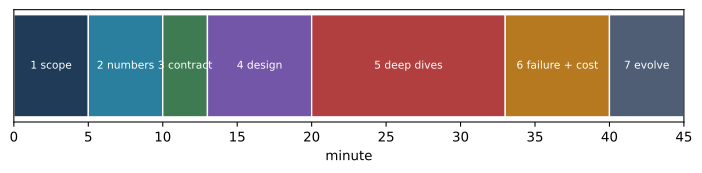
A forty-five-minute design conversation has a shape, and the most common failure is spending its first half in the wrong place. The seven moves below allocate the clock. The minutes are budgets, not stage directions — a real interviewer interrupts, forks, and doubles back — but the ordering is load-bearing: words before numbers, numbers before boxes, boxes before dives, failure before wrap. Table 33.1 is the table this whole Part executes, and Figure 33.1 draws it as a timeline you can rehearse against.

Table 33.1: The seven moves and their minute budgets.

#	Move	Minutes	What seniors do that juniors don’t
1	Scope and the fork question	0–5	Ask the 2–3 clarifiers that change the architecture; state functional and non-functional requirements with numbers; name what is out of scope
2	Back-of-envelope	5–10	Token, KV, QPS, storage, and cost arithmetic before any boxes; the family’s classic numeric trap avoided aloud
3	Contract and SLOs	10–13	The caller-visible API; the SLO split (TTFT versus completion; per-action autonomy tiers); success metrics
4	High-level design	13–20	The family skeleton drawn; every box named with its single responsibility; data and control planes separated
5	Deep dives	20–33	The 2–3 components the interviewer forks into; decisions with alternatives and reasons, not menus
6	Failure, cost, security pass	33–40	The tradeoff table; failure modes with controls; cost and injection treated as attack surfaces; what pages a human
7	Evolution and wrap	40–45	Build order; what to measure first; one changed requirement absorbed without redrawing

import matplotlib.pyplot as plt

moves = [("1 scope", 5), ("2 numbers", 5), ("3 contract", 3), ("4 design", 7),
         ("5 deep dives", 13), ("6 failure + cost", 7), ("7 evolve", 5)]
colors = ["#1f3b57", "#2a7f9e", "#3e7a52", "#7356a8", "#b13f3f", "#b7791f", "#4f5d75"]
fig, ax = plt.subplots(figsize=(7.4, 1.9))
left = 0
for (name, width), color in zip(moves, colors):
    ax.barh(0, width, left=left, color=color, edgecolor="white")
    ax.text(left + width / 2, 0, name, ha="center", va="center", fontsize=8, color="white")
    left += width
ax.set_xlim(0, 45)
ax.set_yticks([])
ax.set_xticks(range(0, 50, 5))
ax.set_xlabel("minute")
fig.tight_layout()
plt.show()

Figure 33.1: Where do the forty-five minutes go? The clock front-loads words and arithmetic: boxes are not drawn until minute 13, and a third of the interview belongs to the deep dives.

We teach the moves against one running prompt, the most-asked design in the agentic loop: “Design question answering over our ten million internal documents. Answers must cite sources, respect per-user permissions, feel instant, and cost pennies.” That sentence is underspecified on purpose — it names no QPS, no freshness requirement, no completion SLO — and the gaps are the interview.

Move 1 — Scope and the fork question. The first five minutes buy information, and the discipline is to ask only questions whose answers change the design. “How many users?” is weak; the load number matters, but it scales boxes rather than choosing them. On the running prompt, the clarifiers that fork the architecture are: do documents change hourly or nightly? — hourly forces an incremental indexing plane, nightly permits a rebuild — and is the assistant read-only, or does it also file tickets? — write-back imports the approval-and-effect machinery of a different family entirely. A senior closes the move by restating the problem with numbers (“ten million documents, call it 50 QPS at peak, p99 feel-instant, a couple of cents per query”) and by naming a non-goal aloud (“no cross-tenant search; out of scope”). Naming what you will not build is a senior signal the rubric explicitly rewards.

Move 2 — Back-of-envelope. Numbers before boxes, always. Four to six anchor numbers are enough: how big is the index, what does one query cost, where does the latency budget go, how many requests are in flight. Each family has one classic numeric trap — for serving designs it is computing KV memory from query heads instead of KV heads — and the senior move is to walk past the trap audibly: “GQA caches eight KV heads, not thirty-two query heads, so this is half a gigabyte per request, not two.” Section 33.3 through Section 33.5 build the calculators that make this move mechanical.

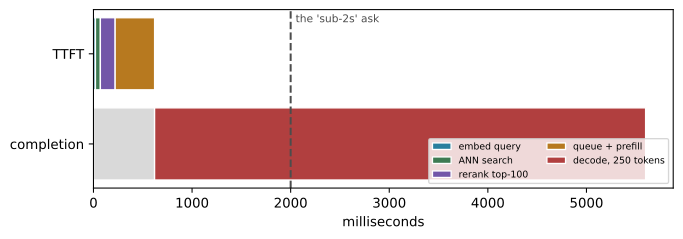
Move 3 — Contract and SLOs. State what the caller sees before designing what is behind it: the API surface in one or two sentences, then the service levels — split correctly. On the running prompt: streamed answers with inline citations; p99 time-to-first-token under 900 ms; completion under 6 s at a 250-token output cap; groundedness above a measured bar on a golden set. The split matters because the two latencies are set by different mechanisms — we compute this in Section 33.3 — and a single “sub-2-seconds” promise is unkeepable in one reading and trivial in the other. When the design takes actions, the contract also states autonomy per action (“reads are automatic, refunds gated”), which Chapter 35 develops.

Move 4 — High-level design. Now the boxes — and the reason the boxes come this late is that the numbers and the contract have already chosen most of them. Draw the family skeleton (Section 33.2), name each box with a single responsibility, and separate the planes: on the running prompt, an asynchronous indexing plane and an online query plane share an index and an ACL store, and confusing them is the classic mid-level error. One sentence per box is enough; the interviewer will choose where to go deeper.

Move 5 — Deep dives. The longest stretch of the clock, and the part that distinguishes deciding from reciting. The interviewer forks into two or three components; for each, the senior pattern is one sentence of recall, then the decision, the alternative, and the reason. On the running prompt: “ACL filtering runs before vector search, not after — post-filtering breaks the top-k guarantee when a user can see 2% of the corpus, and it leaks document existence. The alternative, filter-after-search, is simpler and fine when permissions are coarse; ours are not.” That is a complete dive answer in three sentences. Re-teaching how HNSW works is not a dive; it is a stall.

Move 6 — Failure, cost, security pass. Walk the design as an adversary and as an accountant: which component fails first and what the caller sees; what the tradeoff table looks like (choice, cost, what it buys, risk, control); and the two 2026 defaults — cost is an attack surface (an uncapped loop or an adversarially long query is a denial-of-wallet vector) and retrieved text is data, not instructions (a poisoned document is an injection attempt; Chapter 24 owns the defenses). Close with what pages a human, because a design with no pager story has no operator.

Move 7 — Evolution and wrap. State the build order (“nightly-rebuild index and plain top-k first; rerank and semantic cache only after retrieval metrics justify them”) and what to measure first. Then the interviewer flips one requirement — freshness becomes hourly, the corpus grows tenfold, permissions get row-level — and the senior answer names exactly which boxes change and which survive. Absorbing the flip in two sentences, without redrawing, is the strongest signal the round offers; it demonstrates that the design was a set of reasoned decisions, not a memorized picture.

33.2 The problem-family taxonomy

Every agentic design prompt we have seen in the wild is an instance of one of seven families, and identifying the family in the first minute is what makes the remaining forty-four tractable: the family fixes the skeleton, the classic numeric trap, and the deep dives the interviewer is most likely to fork into. All seven skeletons share one diagram vocabulary — an ingress guard, context assembly (retrieve or observe), the model step (plan or generate), validation, an effect or response, and a record at the end, with a control plane (policy, releases, budgets) and an evidence plane (traces, audits, evals) drawn beside the data path. Families differ in which bone dominates; learning the vocabulary once means every skeleton in Chapters 34–40 reads as a variation, not a new language. Figure 33.2 lays out the seven with the question that identifies each.

flowchart TD
    P["The unseen prompt"] --> A["<b>Retrieval-heavy</b> — Ch 34<br/>Is the hard part locating evidence<br/>under permissions and latency?"]
    P --> B["<b>Acting agents</b> — Ch 35<br/>Does the system change<br/>external state?"]
    P --> C["<b>Model infra</b> — Ch 36<br/>Is the product tokens<br/>served under an SLO?"]
    P --> D["<b>Measurement infra</b> — Ch 37<br/>Is the product a number<br/>someone will trust?"]
    P --> E["<b>State and memory</b> — Ch 38<br/>Must behavior persist<br/>across sessions?"]
    P --> F["<b>Orchestration</b> — Ch 39<br/>Is the work bigger than<br/>one context window?"]
    P --> G["<b>Platform</b> — Ch 40<br/>Are the customers teams,<br/>not end users?"]

Figure 33.2: Which family is this prompt? One identifying question routes an unseen prompt to the family whose skeleton, trap, and deep dives Chapters 34–40 work in full.

Retrieval-heavy (Chapter 34: enterprise RAG; siblings: doc search, visual-document pipelines). The hard part is finding the right evidence at scale, under access control, inside a latency budget. The fork: how fresh must the index be? Nightly rebuild and incremental indexing are different architectures, not different settings. Dominant bone: context assembly; the skeleton is two planes sharing an index.

Acting agents (Chapter 35: support and transactional agents; siblings: browser and computer-use agents). The system changes external state, so authority — not retrieval — is the design center. The fork: which actions are read, compensable, or irreversible? Autonomy is assigned per action, never per agent. Dominant bone: the validate-then-effect path, with approval binding and an effect ledger.

Model infra (Chapter 36: an LLM serving platform). The product is tokens under an SLO, and the design is an argument about accelerator memory and batching. The fork: strict per-request latency or throughput? — it sets the batching policy and everything downstream. Dominant bone: the model step itself; the KV-memory trap lives here.

Measurement infra (Chapter 37: an eval platform). The product is a number that gates launches, so the design question is trust: judge calibration, dataset ownership, statistical honesty. The fork: who owns ground truth? “Correct” is per-team, which makes datasets and judges versioned artifacts. Dominant bone: the evidence plane, promoted to the product.

State and memory (Chapter 38: cross-session memory). Behavior must persist across sessions, so the design is a data model with a security boundary. The fork: what must be remembered — and what must never be? Scope isolation is a correctness property, not a feature. Dominant bone: the record and its read-back path on every turn.

Orchestration (Chapter 39: multi-agent deep research). The work exceeds one context window or one agent’s clock, and the question is whether coordination earns its token multiplier. The fork: is the work read-parallel or write-coupled? Breadth-first reading parallelizes; a single evolving artifact does not, and collapses the design back to one agent with compaction. Dominant bone: the plan step and the merge boundary.

Platform (Chapter 40: a multi-tenant agent platform). The customers are fifty teams, not end users, so the design is governance made mechanical: releases, identity, isolation, evidence. The fork: which controls are mandatory per risk tier, and where is the reviewed escape hatch? Dominant bone: the control plane, promoted to the product.

When a prompt seems to span families — a support agent with heavy retrieval, a platform serving evals — the tiebreak is the fork the interviewer pushes on, and saying so aloud (“this is an acting-agent problem wearing a RAG costume; the risk lives in the refund path, so that is where I will spend the dives”) is itself a senior signal.

33.3 The toolkit: tokens, latency, and dollars

Move 2 is where most candidates go vague, so we now make it mechanical. This section and the next two build the back-of-envelope toolkit as executed code — every calculator is a few lines, every worked example prints its number, and the # @save cells tangle into code/ch33/_generated.py, which Chapters 34–40 import instead of redefining. The point of executing what could be mental arithmetic is honesty: an interview number you have computed twenty times with a tool you built is a number you can produce at a whiteboard without the tool.

Start with money, because it is the arithmetic interviewers ask first. One model call’s cost has three terms — fresh input, cached input, output — and they respond to different knobs, which is why we keep them separate:

C \;=\; \frac{n_{\text{fresh}}\,P_{\text{in}} \;+\; n_{\text{cached}}\,P_{\text{cached}} \;+\; n_{\text{out}}\,P_{\text{out}}}{10^{6}}, \tag{33.1}

where n_{\text{fresh}}, n_{\text{cached}}, and n_{\text{out}} are token counts and each P is a price in dollars per million tokens — the unit vendors quote, which is why the formula divides once at the end rather than trusting us to convert each price by hand.

# @save
from dataclasses import dataclass


@dataclass(frozen=True)
class TokenPrice:
    """Dollar prices for one model, stated per million tokens.

    Interview arithmetic wants prices in the unit vendors quote (dollars per
    million tokens) while formulas want dollars per token. This object stores
    the quoted form and converts exactly once, so a six-order-of-magnitude
    slip cannot hide inside a longer calculation.

    Args:
        input_per_million: Price of one million uncached input tokens.
        output_per_million: Price of one million generated tokens.
        cached_input_per_million: Price of one million input tokens served
            from the provider's prompt cache.
    """

    input_per_million: float
    output_per_million: float
    cached_input_per_million: float = 0.0

    def dollars(self, fresh_in: float, out: float, cached_in: float = 0.0) -> float:
        """Return dollars for one call given its three token counts."""
        return (fresh_in * self.input_per_million
                + cached_in * self.cached_input_per_million
                + out * self.output_per_million) / 1e6


def cost_per_query(input_tokens: int, output_tokens: int, price: TokenPrice,
                   cached_input_tokens: int = 0) -> float:
    """Price one model call from its token counts (@eq-ch33-cost).

    The three terms stay separate because they respond to different knobs:
    fresh input shrinks with context discipline, cached input shrinks the bill
    only if the prompt prefix is stable, and output shrinks only with a length
    cap. The interview move is to say the split aloud — "input dominates at
    this shape, so caching and retrieval width are my cost levers" — before
    naming a total.

    Args:
        input_tokens: All input tokens the call sends, cached or not.
        output_tokens: Generated tokens the call is billed for.
        price: The model's prices per million tokens.
        cached_input_tokens: The part of ``input_tokens`` billed at the
            cached rate.

    Returns:
        Dollars for the call.

    Raises:
        ValueError: If ``cached_input_tokens`` exceeds ``input_tokens``.
    """
    if not 0 <= cached_input_tokens <= input_tokens:
        raise ValueError("cached_input_tokens must lie within input_tokens")
    fresh = input_tokens - cached_input_tokens
    return price.dollars(fresh, output_tokens, cached_input_tokens)

Now the running prompt’s query, priced. A representative shape: a 400-token system prompt plus a 100-token question plus five retrieved 500-token chunks and some history is roughly 3,500 input tokens, with a 250-token cited answer. The prices below are illustrative frontier-class numbers chosen for round arithmetic, not quotes.

price = TokenPrice(input_per_million=3.00, output_per_million=15.00,
                   cached_input_per_million=0.30)
plain = cost_per_query(3_500, 250, price)
warm = cost_per_query(3_500, 250, price, cached_input_tokens=2_500)
print(f"per query, cold cache          : ${plain:.4f}")
print(f"per query, 2.5k-token prefix hot: ${warm:.4f}")
print(f"if peak 50 QPS held for a day  : ${plain * 50 * 86_400:>9,.0f}  vs  ${warm * 50 * 86_400:,.0f}")

per query, cold cache          : $0.0143
per query, 2.5k-token prefix hot: $0.0075
if peak 50 QPS held for a day  : $   61,560  vs  $32,400

About a cent and a half per query meets “cost pennies,” and the day-rate line is the one to say aloud: at peak load the difference between a cold and a warm prompt cache is tens of thousands of dollars per day, which is why cache-aware context assembly (Chapter 13) is a cost decision, not a tidiness preference. The day-rate is an upper bound — real traffic is not flat at peak — and saying that aloud is part of the move.

Latency next. Chapter 1 measured the two phases of one generation and defined TTFT and TPOT (Section 1.6, Equation 1.3); the interview needs one composition on top of them:

T_{\text{complete}} \;=\; T_{\text{TTFT}} \;+\; \left(n_{\text{out}} - 1\right) T_{\text{TPOT}}. \tag{33.2}

# @save
def completion_ms(ttft_ms: float, output_tokens: int, tpot_ms: float) -> float:
    """Return end-to-end latency for one streamed response (@eq-ch33-completion).

    TTFT buys the first token; every later token costs one TPOT. This is why a
    design answer must state two SLOs rather than one: TTFT is set by queueing
    and prefill, completion is set by the output cap, and no amount of
    retrieval tuning moves the second term.

    Args:
        ttft_ms: Time to first token, queueing and prefill included.
        output_tokens: Tokens the response streams.
        tpot_ms: Mean time per output token after the first.

    Returns:
        Milliseconds until the last token arrives; 0.0 for an empty response.
    """
    if output_tokens < 1:
        return 0.0
    return ttft_ms + (output_tokens - 1) * tpot_ms

Chapter 1’s decode simulator gives us a stream to check the composition against — one sentence of recall: simulate_decode produces deterministic token-arrival times for a given prompt and output length, and tpot_ms reads the mean gap off them.

import importlib.util
import sys
from pathlib import Path


def load_chapter(chapter: str, name: str):
    """Import a committed chapter's tangled module under an explicit name."""
    spec = importlib.util.spec_from_file_location(name, Path("code") / chapter / "_generated.py")
    module = importlib.util.module_from_spec(spec)
    sys.modules[name] = module
    spec.loader.exec_module(module)
    return module


ch01 = load_chapter("ch01", "ch01_generated")
times = ch01.simulate_decode(prompt_tokens=800, output_tokens=250)
measured_tpot = ch01.tpot_ms(times)
print(f"simulated stream : TTFT {times[0]:.0f} ms, TPOT {measured_tpot:.2f} ms")
print(f"composed estimate: {completion_ms(times[0], 250, measured_tpot):,.0f} ms")
print(f"last token really arrived at {times[-1]:,.0f} ms")

simulated stream : TTFT 328 ms, TPOT 18.05 ms
composed estimate: 4,823 ms
last token really arrived at 4,823 ms

The composition reproduces the simulated stream exactly, which is the algebra doing its job. Now aim it at the running prompt’s “feel instant.” A representative latency budget for the query path — each stage a number we defend in Chapter 34 — and the completion times it implies:

stages = {"embed query": 20.0, "ANN search": 50.0,
          "rerank top-100": 150.0, "queue + prefill": 400.0}
ttft_budget = sum(stages.values())
print(f"TTFT budget: {ttft_budget:.0f} ms")
for cap in (250, 60):
    print(f"completion at a {cap:3d}-token cap, 20 ms/token: "
          f"{completion_ms(ttft_budget, cap, 20.0):>5,.0f} ms")

TTFT budget: 620 ms
completion at a 250-token cap, 20 ms/token: 5,600 ms
completion at a  60-token cap, 20 ms/token: 1,800 ms

This is the arithmetic behind the SLO split in move 3, and Figure 33.3 draws it. If “instant” means sub-2-seconds to completion, only a 60-token answer qualifies — unusable for a cited paragraph — so the keepable promise is a TTFT SLO with margin plus a completion SLO at a stated output cap. Say the waterfall aloud while you compute it: “620 ms of that budget is pipeline, and the biggest slice is prefill, so context width is my TTFT lever; everything after the first token is the output cap’s problem.”

fig, ax = plt.subplots(figsize=(7.2, 2.6))
stage_colors = ["#2a7f9e", "#3e7a52", "#7356a8", "#b7791f"]
left = 0.0
for (name, width), color in zip(stages.items(), stage_colors):
    ax.barh(1, width, left=left, color=color, edgecolor="white", label=name)
    left += width
ax.barh(0, left, color="0.85", edgecolor="white")
ax.barh(0, completion_ms(left, 250, 20.0) - left, left=left, color="#b13f3f",
        edgecolor="white", label="decode, 250 tokens")
ax.axvline(2_000, ls="--", color="0.3")
ax.text(2_050, 1.35, "the 'sub-2s' ask", fontsize=8, color="0.3")
ax.set_yticks([1, 0])
ax.set_yticklabels(["TTFT", "completion"])
ax.set_xlabel("milliseconds")
ax.legend(loc="lower right", fontsize=7, ncol=2)
fig.tight_layout()
plt.show()

Figure 33.3: Can this design promise ‘sub-2-seconds’? As TTFT, yes, with a 3x margin; as a 250-token completion, never. The SLO must name which latency it bounds — and the output cap it assumes.

NoteLandscape 2026 — the constants in this toolkit

The prices ($3.00 and $15.00 per million tokens, cached input at a tenth), the 20 ms TPOT, the stage latencies, and the 80 GB accelerator used below are illustrative teaching constants chosen for round arithmetic. They move with every pricing page and hardware generation; the formulas do not. Verify live: your provider’s pricing page, your own measured TTFT/TPOT percentiles, and your accelerator’s datasheet before using any of these numbers in a real capacity or budget decision. Checked 2026-07-20.

33.4 The toolkit: memory, throughput, and storage

Three more calculators cover the capacity half of move 2: KV memory, request throughput, and index storage. The first is a recall, not a rebuild — Chapter 3 owns the KV-cache equation and its calculator (Section 3.1, Equation 3.1), and one sentence recaps it: a request’s cache is {2\,L\,H_{kv}\,d_h\,T\,s} bytes — layers times KV heads (not query heads) times head dimension times retained tokens times bytes per scalar, doubled for keys and values. We import it and work the classic 7B-class example, trap included.

ch03 = load_chapter("ch03", "ch03_generated")
gqa = ch03.KVConfig("7B-class GQA-8", layers=32, query_heads=32, kv_heads=8,
                    head_dim=128, bytes_per_scalar=2)
per_request = ch03.kv_bytes(gqa, tokens=4_096)
sixteen = ch03.kv_bytes(gqa, tokens=4_096, batch=16)
trap = sixteen * gqa.query_heads // gqa.kv_heads
print(f"KV, one 4K request      : {per_request / 1e9:.2f} GB  ({per_request / 2**30:.1f} GiB)")
print(f"KV, 16 concurrent       : {sixteen / 1e9:.2f} GB  ({sixteen / 2**30:.0f} GiB)")
print(f"the trap (query heads)  : {trap / 1e9:.2f} GB  -- 4x too high")

KV, one 4K request      : 0.54 GB  (0.5 GiB)
KV, 16 concurrent       : 8.59 GB  (8 GiB)
the trap (query heads)  : 34.36 GB  -- 4x too high

Sixteen concurrent 4K-token requests on a GQA-8 model hold 8.6 GB of cache; compute it from the thirty-two query heads and you get 34 GB and a design sized four times too large. This is the single most reliable numeric trap in serving interviews, and the fix is one audible clause: “GQA caches KV heads, so…”. What the interview then needs is the next step — how many such requests fit on one device — which is a division we make explicit:

# @save
def kv_concurrency_per_device(hbm_bytes: float, weights_bytes: float,
                              kv_bytes_per_request: float,
                              workspace_fraction: float = 0.1) -> int:
    """Return how many requests' KV caches fit on one accelerator.

    Serving capacity is a memory statement before it is a compute statement:
    weights are resident once, a workspace fraction covers activations and
    allocator slack, and the remainder is divided among per-request KV caches.
    The per-request number comes from Chapter 3's calculator
    (@eq-ch03-kvbytes); this function only does the division, so the classic
    trap stays where it belongs — in the KV arithmetic, not here.

    Args:
        hbm_bytes: Device memory in bytes.
        weights_bytes: Resident model weights, after any quantization.
        kv_bytes_per_request: KV payload of one request at its budgeted
            context length.
        workspace_fraction: Fraction of device memory held back for
            activations, fragmentation, and temporaries.

    Returns:
        Whole concurrent requests per device; never negative.

    Raises:
        ValueError: If ``kv_bytes_per_request`` is not positive.
    """
    if kv_bytes_per_request <= 0:
        raise ValueError("kv_bytes_per_request must be positive")
    free = hbm_bytes * (1 - workspace_fraction) - weights_bytes
    return max(int(free // kv_bytes_per_request), 0)

per_device = kv_concurrency_per_device(hbm_bytes=80e9, weights_bytes=16e9,
                                       kv_bytes_per_request=per_request)
print(f"80 GB device, 16 GB fp16 weights, 10% workspace: {per_device} concurrent requests")

80 GB device, 16 GB fp16 weights, 10% workspace: 104 concurrent requests

About a hundred requests per device by memory — an upper bound, since compute and the batching policy (Chapter 10) usually bind first; stating which bound is active is part of the answer. To turn a request rate into a device count we need one bridge between throughput and concurrency, and it is the most quotable formula in the toolkit — Little’s law (Little 1961):

L \;=\; \lambda\,W, \tag{33.3}

where \lambda is arrival rate in requests per second, W is the mean seconds one request stays resident, and L is the mean number of requests in flight. It assumes only a stable system — no distributional fine print — which is what makes it safe to use aloud under pressure.

# @save
import math


def concurrent_requests(qps: float, residence_seconds: float) -> float:
    """Return mean requests in flight via Little's law (@eq-ch33-little).

    Arrival rate times residence time is in-flight work, with no assumptions
    beyond stationarity. In an interview it converts an SLO into a capacity
    statement in one step: cutting residence (a tighter output cap, a faster
    model) shrinks the fleet exactly as effectively as cutting traffic.

    Args:
        qps: Mean arrival rate, requests per second.
        residence_seconds: Mean time one request occupies the system.

    Returns:
        Mean concurrent requests.

    Raises:
        ValueError: If either argument is negative.
    """
    if qps < 0 or residence_seconds < 0:
        raise ValueError("qps and residence_seconds must be nonnegative")
    return qps * residence_seconds


def devices_for_load(qps: float, residence_seconds: float,
                     per_device_concurrency: int, headroom: float = 0.3) -> int:
    """Turn an arrival rate into an accelerator count.

    Little's law gives mean in-flight requests; a headroom factor covers
    burst and tail (the mean is not the p99); dividing by per-device
    concurrency — from :func:`kv_concurrency_per_device` or a measured
    batching limit, whichever is smaller — and rounding up gives devices.

    Args:
        qps: Mean arrival rate, requests per second.
        residence_seconds: Mean residence time per request.
        per_device_concurrency: Concurrent requests one device sustains.
        headroom: Fractional margin above the mean (0.3 = 30%).

    Returns:
        Whole devices, at least 1.

    Raises:
        ValueError: If ``per_device_concurrency`` is not positive.
    """
    if per_device_concurrency < 1:
        raise ValueError("per_device_concurrency must be positive")
    in_flight = concurrent_requests(qps, residence_seconds) * (1 + headroom)
    return max(math.ceil(in_flight / per_device_concurrency), 1)

in_flight = concurrent_requests(qps=50, residence_seconds=5.6)
print(f"50 QPS x 5.6 s residence          = {in_flight:.0f} requests in flight")
print(f"devices at {per_device}/device, 30% headroom: "
      f"{devices_for_load(50, 5.6, per_device)}")
print(f"same, if a 3x burst must be served : {devices_for_load(150, 5.6, per_device)}")

50 QPS x 5.6 s residence          = 280 requests in flight
devices at 104/device, 30% headroom: 4
same, if a 3x burst must be served : 11

The interview framing: “fifty QPS at 5.6 s residence is 280 in flight; with headroom that is four devices, eleven under a three-times burst — so the real design question is whether we buy the burst or shed it.” That last clause is the senior part; the arithmetic exists to set it up. The remaining capacity number is storage for the retrieval index, and its formula is a product of five factors you can recite:

M_{\text{index}} \;=\; n\,d\,b\,i\,r, \tag{33.4}

with n vectors of dimension d at b bytes per element, an index-structure overhead multiplier i, and r replicas. Appendix B’s sizing worksheet carries the same formula in fillable form; here it runs.

# @save
def index_bytes(vectors: int, dim: int, bytes_per_dim: float,
                overhead: float = 1.5, replicas: int = 1) -> float:
    """Size a vector index from first principles (@eq-ch33-index).

    Raw payload is vectors times dimension times element width; a graph or
    codebook structure multiplies it by an overhead factor, and replication
    multiplies again. The result decides a real architecture question — one
    memory-heavy node or a sharded cluster — which is why the number belongs
    in move 2, before any boxes. Source text, metadata, ACL indexes, and
    build-time copies are extra and worth naming aloud.

    Args:
        vectors: Number of stored vectors (chunks, not documents).
        dim: Embedding dimension.
        bytes_per_dim: Element width: 4 for fp32, 2 for fp16, 1 for int8.
        overhead: Index-structure multiplier over raw payload.
        replicas: Full copies serving reads.

    Returns:
        Total bytes across replicas.

    Raises:
        ValueError: If any count is not positive.
    """
    if min(vectors, dim, replicas) < 1 or bytes_per_dim <= 0 or overhead < 1:
        raise ValueError("all sizing factors must be positive (overhead >= 1)")
    return vectors * dim * bytes_per_dim * overhead * replicas

chunks = 30_000_000                      # 10M documents x ~3 chunks each
for label, width in (("fp32", 4), ("int8", 1)):
    total = index_bytes(chunks, dim=1024, bytes_per_dim=width, overhead=1.5, replicas=2)
    print(f"{label}: {total / 1e9:6.1f} GB across 2 replicas "
          f"({total / 2 / 1e9:.1f} GB per copy)")

fp32:  368.6 GB across 2 replicas (184.3 GB per copy)
int8:   92.2 GB across 2 replicas (46.1 GB per copy)

Ten million documents is thirty million chunks, and at fp32 the index is 369 GB — shard it or quantize it, and int8 brings one copy under 50 GB. The chunk-count step is the family’s quiet trap: sizing from documents instead of chunks understates the index threefold, and the correction costs one spoken sentence.

33.5 The toolkit: loop caps and context budgets

Two calculators remain, and they are the two most specific to agentic designs: what a multi-step loop costs, and how a context window is spent. Both look like afterthoughts and both routinely decide interviews, because they are where “the agent will figure it out” meets arithmetic.

An agent loop resends its growing context every step (Chapter 16 built the loop; Chapter 13 owns the assembly). If the context starts at c_0 tokens and grows by g tokens per step — tool results plus the model’s own last output — then across k steps the input tokens sum to

N_{\text{in}}(k) \;=\; k\,c_0 \;+\; g\,\frac{k\,(k-1)}{2}, \tag{33.5}

which is quadratic in k: each step looks cheap, and the sum does not. The calculator prices the loop under Equation 33.1, with and without a prompt cache over the resent prefix.

# @save
def loop_cost(steps: int, base_context_tokens: int, growth_tokens_per_step: int,
              output_tokens_per_step: int, price: TokenPrice,
              cached_resend: bool = False) -> float:
    """Price an agent loop that resends its growing context (@eq-ch33-loop).

    Step ``i`` sends the whole context so far — base plus ``i - 1`` growth
    increments — so uncached input cost grows quadratically in steps even
    though each single step looks cheap. With ``cached_resend`` the previous
    step's context is billed at the cached rate and only the new tokens are
    fresh, which is the mechanism that makes long loops affordable. Either
    way, the honest design move is a hard step cap with an escalation path,
    priced in advance.

    Args:
        steps: Loop iterations to price.
        base_context_tokens: Context at step one (system, tools, task).
        growth_tokens_per_step: Tokens appended per step (tool results plus
            the previous output).
        output_tokens_per_step: Tokens generated at each step.
        price: The model's prices per million tokens.
        cached_resend: Bill each step's previously-sent prefix at the cached
            rate instead of the fresh rate.

    Returns:
        Dollars for the whole loop.

    Raises:
        ValueError: If ``steps`` is not positive or any count is negative.
    """
    if steps < 1 or min(base_context_tokens, growth_tokens_per_step,
                        output_tokens_per_step) < 0:
        raise ValueError("steps must be positive and token counts nonnegative")
    total = 0.0
    for i in range(1, steps + 1):
        context = base_context_tokens + (i - 1) * growth_tokens_per_step
        cached = context - growth_tokens_per_step if (cached_resend and i > 1) else 0
        total += cost_per_query(context, output_tokens_per_step, price,
                                cached_input_tokens=cached)
    return total


def max_affordable_steps(budget_dollars: float, base_context_tokens: int,
                         growth_tokens_per_step: int, output_tokens_per_step: int,
                         price: TokenPrice, cached_resend: bool = False,
                         step_cap: int = 1_000) -> int:
    """Return the largest step count whose loop cost fits a budget.

    This is the loop cap stated as money instead of a guess: given a per-task
    budget, it walks steps upward until the next one would break the budget.
    A returned 0 means even one step exceeds the budget — a design signal,
    not an edge case.

    Args:
        budget_dollars: The per-task spend ceiling.
        base_context_tokens: Context at step one.
        growth_tokens_per_step: Tokens appended per step.
        output_tokens_per_step: Tokens generated per step.
        price: The model's prices per million tokens.
        cached_resend: Whether resent prefixes bill at the cached rate.
        step_cap: Safety bound on the search.

    Returns:
        The largest affordable whole number of steps, up to ``step_cap``.
    """
    affordable = 0
    for k in range(1, step_cap + 1):
        if loop_cost(k, base_context_tokens, growth_tokens_per_step,
                     output_tokens_per_step, price, cached_resend) > budget_dollars:
            break
        affordable = k
    return affordable

A representative acting-agent shape: 2,000 tokens of system prompt and tool schemas, 800 tokens added per step, 300 generated per step.

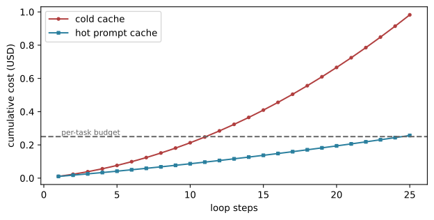
for k in (5, 10, 20):
    cold = loop_cost(k, 2_000, 800, 300, price)
    hot = loop_cost(k, 2_000, 800, 300, price, cached_resend=True)
    print(f"{k:2d} steps: ${cold:.3f} cold cache   ${hot:.3f} hot cache")
budget = 0.25
print(f"\nsteps a ${budget:.2f} budget buys: "
      f"{max_affordable_steps(budget, 2_000, 800, 300, price)} cold, "
      f"{max_affordable_steps(budget, 2_000, 800, 300, price, cached_resend=True)} hot")

 5 steps: $0.076 cold cache   $0.042 hot cache
10 steps: $0.213 cold cache   $0.087 hot cache
20 steps: $0.666 cold cache   $0.194 hot cache

steps a $0.25 budget buys: 11 cold, 24 hot

Twenty cold steps cost well over three times what twenty hot steps do, and a 25-cent budget buys eleven steps cold versus more than twice as many hot — Figure 33.4 draws both curves against that budget line. The interview framing has two halves: “loop cost is quadratic in steps unless the prefix caches, so my cost controls are a hard step cap with escalation, and cache-stable context assembly” — and, from move 6, “the cap is also a security control, because an adversary who can extend the loop is spending my money” (the denial-of-wallet framing Chapter 26 develops).

steps_axis = list(range(1, 26))
cold_curve = [loop_cost(k, 2_000, 800, 300, price) for k in steps_axis]
hot_curve = [loop_cost(k, 2_000, 800, 300, price, cached_resend=True) for k in steps_axis]
fig, ax = plt.subplots(figsize=(6.6, 3.4))
ax.plot(steps_axis, cold_curve, marker="o", ms=3, color="#b13f3f", label="cold cache")
ax.plot(steps_axis, hot_curve, marker="s", ms=3, color="#2a7f9e", label="hot prompt cache")
ax.axhline(0.25, ls="--", color="0.4")
ax.text(1.2, 0.26, "per-task budget", fontsize=8, color="0.4")
ax.set_xlabel("loop steps")
ax.set_ylabel("cumulative cost (USD)")
ax.legend()
fig.tight_layout()
plt.show()

Figure 33.4: What does an agent loop cost as it runs longer? Cold-cache cost bends upward (quadratic resend); a hot prompt cache keeps it near-linear. The dashed line is a 25-cent per-task budget — the step cap made visible.

The last calculator is the humblest and the one that catches overcommitted designs fastest: the context window is an account, and the design must balance it. System prompt, kept history, retrieved evidence, and a reserved output allocation must fit inside the window with slack:

W_{\text{ctx}} \;=\; n_{\text{sys}} + n_{\text{hist}} + n_{\text{ret}} + n_{\text{reserve}} + n_{\text{free}}, \qquad n_{\text{free}} \ge 0, \tag{33.6}

where W_{\text{ctx}} is the window and the components are the token allocations just named. The reserve matters because generation that runs out of window is truncated output, a user-visible failure; the free term matters because a plan that lands at exactly zero has no room for the next tool result.

# @save
def context_budget(window_tokens: int, *, system: int, history: int,
                   retrieval: int, output_reserve: int) -> dict[str, int]:
    """Balance one call's context window like an account (@eq-ch33-context).

    The window is a hard capacity shared by everything the call sends and
    reserves; this function makes the split explicit and refuses an
    overcommitted plan instead of letting truncation decide silently at
    runtime. Saying the split aloud is the fastest way to expose a design
    error — a 40k-token retrieval plan inside a 32k window is a redesign,
    not a tuning problem. Chapter 13 owns what to do when the budget stops
    fitting: compact deliberately rather than truncate accidentally.

    Args:
        window_tokens: The model's context window.
        system: Tokens for instructions and tool schemas.
        history: Conversation or trajectory tokens kept verbatim.
        retrieval: Retrieved or observed evidence tokens.
        output_reserve: Tokens reserved so generation cannot be cut off.

    Returns:
        A dict of the four components plus ``"free"``, the uncommitted slack.

    Raises:
        ValueError: If the window is not positive, a component is negative,
            or the components exceed the window.
    """
    parts = {"system": system, "history": history,
             "retrieval": retrieval, "output_reserve": output_reserve}
    if window_tokens < 1 or any(v < 0 for v in parts.values()):
        raise ValueError("window must be positive and components nonnegative")
    used = sum(parts.values())
    if used > window_tokens:
        raise ValueError(f"overcommitted by {used - window_tokens:,} tokens")
    return {**parts, "free": window_tokens - used}

plan = context_budget(128_000, system=3_000, history=45_000,
                      retrieval=12_000, output_reserve=4_000)
print("128k plan:", plan)
try:
    context_budget(32_000, system=3_000, history=18_000,
                   retrieval=40_000, output_reserve=2_000)
except ValueError as err:
    print("32k plan :", err)

128k plan: {'system': 3000, 'history': 45000, 'retrieval': 12000, 'output_reserve': 4000, 'free': 64000}
32k plan : overcommitted by 31,000 tokens

The second call is the teaching moment: the same retrieval ambition that fits comfortably in a 128k window overcommits a 32k one by 31,000 tokens, and the calculator refuses it at design time instead of letting the runtime truncate the evidence. In the interview this arithmetic takes fifteen seconds and buys a claim few candidates can make: “here is my context budget, and here is the free headroom the next tool result lands in.”

33.6 How you are graded

The rubric behind this round is not a secret, and this book keeps exactly one copy of it: Appendix B’s five-layer review rubric — scope and contract, model and data path, authority and security, reliability and economics, evidence and operations — with its 45-minute protocol and 0–4 self-scoring scale and its scoping form. We do not restate them here; we use them. The seven moves are that rubric turned into a clock: moves 1–3 earn layer one, move 4 earns layer two, the dives and the failure pass earn layers three and four, and move 7 earns layer five. The scoring is AND-gated — a brilliant retrieval dive does not compensate for a design with no authority story — which is why the clock refuses to let any move be skipped. What changes between candidate levels is not which topics come up but what the interviewer hears when they do (Table 33.2):

Table 33.2: Signals per level: the same topics, heard differently.

Level	What the interviewer hears
Junior	Components named and wired in a generic diagram; numbers absent, asserted, or in the wrong unit; dives that explain how a mechanism works rather than choose one; the changed requirement triggers a redraw
Senior	The forks asked first; four to six anchor numbers computed before boxes; every dive shaped as decision, alternative, reason; failure and cost priced; the changed requirement absorbed in two sentences
Staff	All of the senior signals, plus the prompt’s own frame challenged when it deserves it; what will not be built stated with reasons; every control tied to an operating cost and an owner; the build order defended as an evidence-gathering sequence

Five anti-patterns account for most failed senior rounds, and each has a one-sentence fix.

• Architecture-first. Boxes at minute two mean every later number must be retrofitted to a drawing; the fix is the clock itself — nothing is drawn before minute 13, however strong the urge.
• No numbers. A design defended entirely in adjectives (“fast”, “scalable”) cannot survive move 5; the fix is drilling the six calculators in this chapter until the input shapes are memorized, because the interviewer supplies the inputs and the procedure produces the number.
• One lucky trace. Walking a single happy-path request and calling the design validated; the fix is pairing every normal-path walk with the two failure paths move 6 demands — what breaks first, and what the caller sees when it does.
• Re-teaching instead of deciding. Spending a dive explaining how HNSW or continuous batching works; the fix is the three-sentence dive shape — one sentence of recall, then the decision, the alternative, and the reason.
• Ignoring the changed requirement. Treating move 7’s flip as an attack on the design rather than the point of it; the fix is answering with the delta — which boxes change, which survive — which is precisely the skill the family-skeleton tables in Chapters 34–40 train.

A useful drill loop, which Appendix B’s self-scoring section formalizes: run a prompt against the clock, score the five layers 0–4, and treat any layer at 2 or below as a pointer back to its owning chapter — not to this Part, which assembles arguments, but to the spine chapter that teaches the mechanism the argument needed.

33.7 Running the clock

We close by running the whole procedure once, compressed, on the running prompt — question answering over ten million internal documents; cited, permissioned, instant-feeling, pennies — as a preview of the shape every following chapter works in full. Chapter 34 runs this same prompt at interview depth; here each move gets a paragraph, so the choreography is visible end to end.

Minutes 0–5, scope. Two fork questions: documents change nightly (a rebuild is legal), and the assistant is read-only (no effect machinery). Requirements restated with numbers: ten million documents, peak 50 QPS, p99 TTFT under 900 ms, completion under 6 s at a 250-token cap, roughly two cents a query, per-user ACLs enforced strictly, every claim cited. Out of scope, said aloud: cross-tenant search, write-back, freshness under a day.

Minutes 5–10, back-of-envelope. The anchor numbers, straight from the toolkit — this cell is the interview’s whiteboard arithmetic, executed:

anchors = [
    ("index: 30M chunks, int8, x1.5, x2 replicas",
     f"{index_bytes(30_000_000, 1024, 1, 1.5, 2) / 1e9:,.0f} GB"),
    ("TTFT budget (embed+ANN+rerank+prefill)", f"{ttft_budget:,.0f} ms"),
    ("completion at the 250-token cap",
     f"{completion_ms(ttft_budget, 250, 20.0) / 1000:.1f} s"),
    ("cost per query, warm prompt cache",
     f"${cost_per_query(3_500, 250, price, cached_input_tokens=2_500):.4f}"),
    ("in flight at 50 QPS (Little's law)",
     f"{concurrent_requests(50, 5.6):.0f} requests"),
    ("generation devices, 30% headroom", f"{devices_for_load(50, 5.6, per_device)}"),
]
for name, value in anchors:
    print(f"{name:44} {value}")

index: 30M chunks, int8, x1.5, x2 replicas   92 GB
TTFT budget (embed+ANN+rerank+prefill)       620 ms
completion at the 250-token cap              5.6 s
cost per query, warm prompt cache            $0.0075
in flight at 50 QPS (Little's law)           280 requests
generation devices, 30% headroom             4

Six numbers in five minutes, each one sentence of narration: the index fits two commodity replicas at int8; TTFT has a 900 ms budget with 280 ms of margin over the 620 ms waterfall; completion honesty forces the output cap into the SLO; the query price meets “pennies” because the prefix caches; and the serving fleet is four devices, not forty. The trap avoided aloud: chunks, not documents, size the index.

Minutes 10–13, contract. One endpoint: streamed answer plus citation list, answerable=false as a first-class result (abstention is a feature, recall Section 1.4). SLOs as computed above; success metrics: groundedness and citation-precision on a golden set, measured weekly, with the abstention rate watched alongside so the system cannot buy groundedness by refusing everything.

Minutes 13–20, high-level design. The retrieval-heavy skeleton, Figure 33.5: an asynchronous indexing plane (chunk, embed, build) and an online query plane (embed, ACL-prefilter, ANN search, rerank, pack, generate-with-citations, validate) sharing the index and the ACL store. Every box has one responsibility; the two planes meet only at the index swap, which is versioned so a bad build rolls back by pointer flip.

flowchart LR
    subgraph IDX ["indexing plane — async, nightly"]
        S["sources"] --> CH["chunk + embed"] --> B["build + validate"]
    end
    B --> IX[("versioned ANN index<br/>+ metadata / ACL store")]
    subgraph QRY ["query plane — online, 620 ms budget"]
        Q["query"] --> E2["embed"] --> F["ACL prefilter"] --> A2["ANN top-100"]
        A2 --> RR["rerank top-5"] --> PK["pack context"] --> G["generate + cite"] --> V["validate / abstain"]
    end
    IX --> F

Figure 33.5: The retrieval-heavy family skeleton for the enterprise-RAG prompt: where does work happen off the hot path, and where must every online millisecond be defended? Chapter 34 works every box at interview depth.

Minutes 20–33, deep dives. The two forks this prompt reliably produces: permissions (filter before search; the alternative and its breaking point argued as in move 5 above) and the rerank stage (a cross-encoder buys precision at 150 ms and a device; the alternative — wider top-k into the packer — is cheaper and worse, and the decision is owned by a measured recall-versus-latency curve, not taste). A third dive the interviewer may take is the semantic cache, and its risk — serving a stale or wrongly-scoped answer — is why the cache key must include the ACL scope.

Minutes 33–40, failure, cost, security. What breaks first: the reranker under burst (control: shed to no-rerank mode, which degrades precision measurably instead of availability); a poisoned document carrying injected instructions (retrieved text is data — delimited, provenance-tagged; Chapter 24’s architecture); a mis-scoped ACL entry (the one failure with no partial credit — negative isolation tests in CI, and a leak pages a human immediately). Cost as attack surface: query length capped, per-user rate limits, the day-rate arithmetic from Section 33.3 quoted as the reason.

Minutes 40–45, evolution. Build order: nightly index, plain top-k, no rerank, no cache — measure retrieval recall first, because it caps everything downstream (Chapter 14’s lesson). Add the reranker when the recall curve says so; add the semantic cache when the traffic histogram says so. Then the flip lands — “documents now change hourly” — and the answer is the delta: the indexing plane becomes incremental with a freshness watermark the query plane checks; the query plane, the contract, and five of the six anchor numbers do not move. That sentence — what changes, what survives — is the interview’s real finish line, and it is where every chapter in this Part will end.

33.8 Summary

The agentic system-design round grades a procedure, and this chapter built it: seven moves on a 45-minute clock (words, then numbers, then boxes, then decisions, then failure, then the flip), a seven-family taxonomy whose identifying questions route any unseen prompt, and an executed back-of-envelope toolkit — cost, completion latency, KV-derived concurrency, Little’s-law fleets, index sizing, loop caps, context budgets — that turns move 2 into mechanics. Grading lives in Appendix B’s five-layer rubric; the anti-patterns are all failures of ordering or arithmetic. Chapter 34 now runs the first family, enterprise RAG, at full interview depth.

33.9 Exercises

1. Route three prompts. For each of (a) “design a voice concierge for a hotel chain,” (b) “design a text-to-SQL analytics assistant over our warehouse,” and (c) “design the system that decides whether our support agent is safe to ship each week” — name the family, the identifying question that told you, and the first fork you would ask. One of the three is a deliberate costume; say which and why.
2. Move 2 on unfamiliar ground. Apply move 2 to “design a nightly batch service that summarizes two million support tickets”: choose four anchor numbers, compute them with this chapter’s calculators (batch has no TTFT — which number replaces it?), and name the numeric trap you avoided.
3. Push the cost model. Using cost_per_query and the chapter’s illustrative prices: (a) quadruple the output cap to 1,000 tokens and report which term dominates the query price now; (b) find the cached-input fraction at which the 3,500-in/250-out query drops below one cent; (c) using max_affordable_steps, find the largest per-step growth g that keeps a 20-step hot-cache loop under $0.20.
4. Work the trap in both directions. Recompute the sixteen-request fleet number from Section 33.4 deliberately using query heads, state the ratio to the correct number, and explain in one sentence why GQA caches only H_{kv} (recall Section 3.1). Then replace the config with an MLA-style cache (latent rank 512, decoupled rotary key 64) and report what happens to kv_concurrency_per_device.
5. Buy the burst or shed it. Peak triples to 150 QPS. Recompute in-flight requests and devices; then instead hold 50 QPS but cut the output cap to 100 tokens, recompute residence via Equation 33.2 and the fleet again. State which knob you would pull first and what it costs the user.
6. Watch a budget die. An agent runs in a 32k window with a 4,000-token system prompt, history growing 1,200 tokens per turn, 3,000 tokens of retrieval per turn, and a 2,000-token output reserve. Using context_budget, find the turn at which the plan overcommits, then propose the compaction policy (Chapter 13) that extends it and show the new arithmetic.
7. Run the clock for real. Take design H from Appendix B’s prompt table (the self-hosted model platform), set a 45-minute timer, and run all seven moves against Figure 33.1. Score yourself with Appendix B’s 0–4 self-scoring table, log the minute at which each move actually started against its budget, and route your weakest layer to its owning chapter.

Little, John D. C. 1961. “A Proof for the Queuing Formula: L = \lambda W.” Operations Research 9 (3): 383–87.