flowchart LR
    U(["request: prompt, SLO"]) --> G["gateway: admit"]
    G --> R["KV- and load-aware router"]
    R --> S["iteration scheduler"]
    S --> E(["engine and kernels"])
    E <--> K[("paged KV pool")]
    E --> D["detokenize and stream"]
    D --> U
    S -.->|"queue, preemption"| M[["measurements"]]
    K -.->|"hits, evictions"| M
    D -.->|"TTFT, token gaps"| M
10 Serving at Scale: Engines, Caching, Quantization, and Production Test-Time Compute
We are now ready to turn one model’s forward pass into a service that many callers share at once, and to measure every trade that turn requires. We build one deterministic serving lab, in fragments, across the chapter: a load sweep that shows throughput and goodput diverging; a continuous-batching scheduler that fills the holes a fixed batch leaves; a paged-memory allocator that reclaims the fragmentation a contiguous KV cache strands; a prefix cache with a hit-rate break-even; a speculative-decoding model whose speedup we sweep against acceptance rate; an honest int8 quantization of the tiny GPT we trained in Chapter 2, measured for size and drift; a grammar mask applied to that model’s real logits; and a reasoning-budget sweep that shows accuracy saturating while tokens keep accruing. Each mechanism recalls something earlier: the KV-cache arithmetic of Chapter 3, the two latency phases of a request from Chapter 9, and the marginal-value view of extra compute from Chapter 8. Serving is where those mechanisms meet contention.
The lab is a CPU simulation with synthetic workloads and one small real model. It validates equations and decision logic; it does not benchmark an accelerator, an engine, or a provider. Every number below is reproduced by the cell that prints it.
10.1 Goodput is the number a serving system optimizes
A model endpoint reports record token throughput after a deployment change. At the same time, interactive users see more long pauses before the first token, and streaming freezes behind large prompts. Both observations are true. The server completed more work per second by accepting larger batches, but too many individual requests missed their latency contract. Throughput rewarded work that users experienced as late.
The objective that resolves the contradiction is goodput: the rate of requests that finish while satisfying every declared service-level objective (SLO). Let a window of W seconds contain requests indexed by i, each with a time to first token T_i^{\text{first}} and a time per output token T_i^{\text{token}}, against limits S^{\text{first}} and S^{\text{token}}. Two-SLO goodput is
G = \frac{1}{W}\sum_i \mathbf{1}\!\left[T_i^{\text{first}}\le S^{\text{first}}\ \wedge\ T_i^{\text{token}}\le S^{\text{token}}\right]\quad\text{requests/second.} \tag{10.1}
The indicator contributes one only when both conditions hold. Reporting each pass rate separately hides that different requests fail each objective; the conjunction is the point. Time to first token and time per output token keep their boundaries from Chapter 9 — end-to-end TTFT includes admission, queueing, tokenization, prefill, and the first decode step, so a fast isolated forward pass does not imply a fast service.
Goodput is a function of offered load. Figure 10.1 locates where load turns into latency: every component on the path can add queueing or change a request’s state.
To see goodput and throughput diverge we build a small slot-based simulator. Requests arrive as a Poisson process at rate rate; the server holds slots decode streams and advances one step per unit time; a waiting request queues until a slot frees. Its queue wait is a proxy for TTFT. This is the systems analogue of training a model and plotting the loss: we drive the mechanism with a synthetic workload and read the curve it produces.
# @save
import numpy as np


def sweep_load(rates, slots=8, mean_service=20.0, ttft_slo=30,
               horizon=4000, seed=0):
    """Measure throughput and goodput of a slot server across arrival rates.

    A fixed pool of ``slots`` decode streams advances one step per unit time.
    Requests arrive by a Poisson process; each waits in a FIFO queue for a free
    slot, and its queue wait is charged as time-to-first-token. Goodput counts
    only completions whose admission delay met ``ttft_slo``, so it can fall even
    as throughput climbs toward the pool's capacity of ``slots / mean_service``
    requests per step (@eq-ch10-goodput).

    Args:
        rates: Arrival rates (requests per step) to sweep.
        slots: Concurrent decode streams the server can run.
        mean_service: Mean decode length; service is uniform on ``[1, 2*mean)``.
        ttft_slo: Admission-delay budget, in steps, that a completion must meet.
        horizon: Simulated steps per rate.
        seed: Seed for the arrival and service draws.

    Returns:
        One dict per rate with ``throughput``, ``goodput`` (both per step), and
        the ``qualified`` fraction of completions that met the SLO.
    """
    rows = []
    rng = np.random.default_rng(seed)
    for rate in rates:
        gaps = rng.exponential(1.0 / rate, size=int(rate * horizon * 1.4) + 100)
        arrivals = np.floor(np.cumsum(gaps)).astype(int)
        arrivals = arrivals[arrivals < horizon]
        service = rng.integers(1, 2 * int(mean_service), size=len(arrivals))
        active, queue, done, ok, cursor = [], [], 0, 0, 0
        for step in range(horizon):
            while cursor < len(arrivals) and arrivals[cursor] == step:
                queue.append((int(arrivals[cursor]), int(service[cursor])))
                cursor += 1
            active = [(fin, arr) for (fin, arr) in active if fin > step]
            while queue and len(active) < slots:
                arrival, length = queue.pop(0)
                ok += (step - arrival) + 1 <= ttft_slo
                active.append((step + length, arrival))
                done += 1
        rows.append({"rate": rate, "throughput": done / horizon,
                     "goodput": ok / horizon, "qualified": ok / max(1, done)})
    return rows
The pool’s capacity is slots / mean_service = 8 / 20 = 0.4 requests per step. We sweep from well below to twice that and print the two rates side by side.
capacity = 8 / 20.0
rates = [round(capacity * f, 3) for f in (0.3, 0.5, 0.7, 0.85, 1.0, 1.15, 1.35, 1.6, 2.0)]
knee = sweep_load(rates)
print(f"{'rate':>6} {'throughput':>11} {'goodput':>8} {'qualified':>10}")
for row in knee:
    print(f"{row['rate']:>6} {row['throughput']:>11.3f} "
          f"{row['goodput']:>8.3f} {row['qualified']:>10.3f}")
rate throughput goodput qualified
0.12 0.107 0.107 1.000
0.2 0.194 0.194 1.000
0.28 0.275 0.275 1.000
0.34 0.359 0.324 0.903
0.4 0.398 0.126 0.316
0.46 0.392 0.017 0.043
0.54 0.399 0.015 0.038
0.64 0.399 0.010 0.025
0.8 0.400 0.005 0.014Throughput rises with load and then flattens at the capacity of 0.4: the server never completes more than it can. Goodput does something else entirely. It climbs while the queue stays short, peaks near 0.32 just below capacity, then collapses as the queue explodes — at the highest rate, the server is fully busy yet almost no completion meets its SLO. That gap between the two curves, drawn in Figure 10.2, is the whole subject of the chapter.
Show the code that draws this figure
import matplotlib.pyplot as plt

xs = [r["rate"] for r in knee]
fig, ax = plt.subplots(figsize=(6.6, 3.6))
ax.plot(xs, [r["throughput"] for r in knee], "s-", color="#2a7f9e", label="throughput")
ax.plot(xs, [r["goodput"] for r in knee], "o-", color="#b13f3f", label="goodput (SLO-qualified)")
ax.axhline(0.4, ls="--", color="#555", lw=1)
ax.axvline(xs[knee.index(max(knee, key=lambda r: r["goodput"]))], ls=":", color="#b13f3f", lw=1)
ax.set_xlabel("offered load (requests / step)")
ax.set_ylabel("completions / step")
ax.legend()
fig.tight_layout()
plt.show()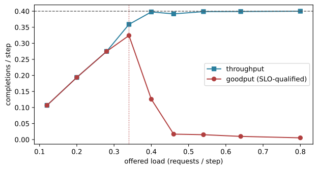
Capacity is therefore not a single number but this curve, pinned to a workload: token lengths, concurrency, cancellations, cache pattern, and decoding policy all move the knee. Chapter 26 owns monetary cost and fleet provisioning; this chapter supplies the mechanics that set where the knee sits. Every optimization that follows is an attempt to push the red curve right without letting it fall.
NoteIn the interview
Q. Your dashboard shows record tokens per second after a batching change, but users are complaining. What do you measure, and what is likely wrong?
A. Report goodput, not throughput: the fraction of requests meeting TTFT and TPOT, per SLO, as a function of offered load. Larger batches raised throughput by pushing the system past the goodput knee — queue wait and preemption now break the latency contract for many requests. The trap is reporting mean latency; the tail is where the SLO fails, so show the qualified fraction and the p99 inter-token gap.
10.2 Continuous batching and paged KV turn variation into schedulable work
A fixed batch of four decode requests has remaining lengths 2, 12, 4, and 10 tokens. After the two-token request finishes, its slot sits idle until the twelve-token request finishes. Compute is stranded not because the server is slow but because variable-length requests are being treated as one fixed rectangle. For a static batch of size B with output lengths L_1,\dots,L_B, slot utilization is
U_{\text{static}}=\frac{\sum_{i=1}^{B}L_i}{B\max_i L_i}, \tag{10.2}
the useful request-steps over the slots held while the longest member runs. Length skew drives it down. Continuous batching, also called iteration-level or in-flight batching, makes admission a per-step decision: after each decode step the scheduler removes finished requests and admits waiting ones into the freed slots (Yu et al. 2022). We implement both policies and compare them on one burst of twelve requests into four slots.
# @save
REQUEST_LENGTHS = [2, 12, 4, 10, 3, 9, 5, 8, 6, 7, 2, 11]


def static_schedule(lengths, batch_size):
    """Run fixed batches that each wait for their longest member to finish.

    Requests are grouped in arrival order; a group occupies all ``batch_size``
    slots until its longest member completes, so short members leave idle slots
    (the loss @eq-ch10-ustatic quantifies).

    Args:
        lengths: Decode length of each request, in steps.
        batch_size: Number of slots the batch fills.

    Returns:
        A dict of per-request ``starts`` and ``finishes``, the total
        ``makespan_steps``, and slot ``utilization``.
    """
    starts, finishes, elapsed = [0] * len(lengths), [0] * len(lengths), 0
    for base in range(0, len(lengths), batch_size):
        group = lengths[base:base + batch_size]
        for offset, length in enumerate(group):
            starts[base + offset] = elapsed
            finishes[base + offset] = elapsed + length
        elapsed += max(group)
    return {"starts": starts, "finishes": finishes, "makespan_steps": elapsed,
            "utilization": sum(lengths) / (batch_size * elapsed)}
The continuous scheduler keeps a waiting queue and refills a slot the instant its request completes, so a finished short request is immediately replaced rather than leaving a hole.
# @save
def continuous_schedule(lengths, batch_size):
    """Refill each decode slot as soon as its current request completes.

    Admission is decided every step: finished requests leave and waiting ones
    enter the freed slots, so slot occupancy stays near ``batch_size`` until the
    queue drains. This is iteration-level batching; its win over
    ``static_schedule`` is the point of @eq-ch10-ustatic.

    Args:
        lengths: Decode length of each request, in steps.
        batch_size: Number of concurrent slots.

    Returns:
        A dict of per-request ``starts`` and ``finishes``, the total
        ``makespan_steps``, and slot ``utilization``.
    """
    starts, finishes = [-1] * len(lengths), [-1] * len(lengths)
    remaining, active, waiting, step = lengths[:], [], list(range(len(lengths))), 0
    while waiting and len(active) < batch_size:
        request = waiting.pop(0); starts[request] = step; active.append(request)
    used = 0
    while active:
        used += len(active)
        for request in active:
            remaining[request] -= 1
        step += 1
        for request in [r for r in active if remaining[r] == 0]:
            finishes[request] = step; active.remove(request)
        while waiting and len(active) < batch_size:
            request = waiting.pop(0); starts[request] = step; active.append(request)
    return {"starts": starts, "finishes": finishes, "makespan_steps": step,
            "utilization": used / (batch_size * step)}
Goodput needs an SLO test per request. We charge time to first token as the admission step plus one, and time per output token as elapsed steps over tokens produced. With a TTFT budget of 16 steps and a TPOT budget of 1.05, we count how many requests qualify under each policy.
# @save
def goodput(schedule, lengths, ttft_slo=16, tpot_slo=1.05):
    """Count requests meeting both latency SLOs, and the per-step goodput.

    A request qualifies when its admission delay is within ``ttft_slo`` and its
    steps-per-token stays within ``tpot_slo``. This is @eq-ch10-goodput applied
    to a finished schedule, and it is what separates the two policies even when
    both eventually complete every request.

    Args:
        schedule: A dict from ``static_schedule`` or ``continuous_schedule``.
        lengths: Decode length of each request, in steps.
        ttft_slo: Admission-delay budget, in steps.
        tpot_slo: Time-per-output-token budget, in steps.

    Returns:
        A dict with the ``qualified`` count and ``per_step`` goodput.
    """
    qualified = 0
    for start, finish, length in zip(schedule["starts"], schedule["finishes"], lengths):
        if start + 1 <= ttft_slo and (finish - start) / length <= tpot_slo:
            qualified += 1
    return {"qualified": qualified, "per_step": qualified / schedule["makespan_steps"]}
We run both policies on the burst and print makespan, utilization, and goodput.
static = static_schedule(REQUEST_LENGTHS, 4)
continuous = continuous_schedule(REQUEST_LENGTHS, 4)
for name, sched in (("static", static), ("continuous", continuous)):
    g = goodput(sched, REQUEST_LENGTHS)
    print(f"{name:>11}: makespan {sched['makespan_steps']:>2}  "
          f"util {sched['utilization']:.3f}  qualified {g['qualified']:>2}/12  "
          f"goodput {g['per_step']:.3f}")
static: makespan 32 util 0.617 qualified 8/12 goodput 0.250
continuous: makespan 26 util 0.760 qualified 12/12 goodput 0.462Continuous batching finishes the burst in 26 steps instead of 32, lifts utilization from 0.62 to 0.76, and — the number that matters — qualifies all twelve requests instead of eight. To see why four requests fail under static batching, print their admission steps.
print("static admission steps:    ", static["starts"])
print("continuous admission steps:", continuous["starts"])
static admission steps: [0, 0, 0, 0, 12, 12, 12, 12, 21, 21, 21, 21]
continuous admission steps: [0, 0, 0, 0, 2, 4, 5, 10, 10, 12, 13, 15]Under static batching the third group of four requests is not admitted until step 21, so its time to first token is 22 — past the 16-step budget. Those four requests complete, but late. Continuous batching admits its last request at step 15, inside the budget. The holes the fixed batch leaves are exactly the requests that miss the SLO. Figure 10.3 shades them.
Show the code that draws this figure
def slot_rows(sched, batch_size):
    rows = [[] for _ in range(batch_size)]
    order = sorted(range(len(REQUEST_LENGTHS)), key=lambda i: (sched["starts"][i], i))
    free = list(range(batch_size))
    busy = {}
    for i in sorted(order, key=lambda i: sched["starts"][i]):
        s, f = sched["starts"][i], sched["finishes"][i]
        for slot, end in list(busy.items()):
            if end <= s:
                free.append(slot); del busy[slot]
        slot = free.pop(0); busy[slot] = f
        rows[slot].append((i, s, f))
    return rows

fig, axes = plt.subplots(2, 1, figsize=(7.2, 3.8), sharex=True)
for ax, (title, sched) in zip(axes, [("static batching", static), ("continuous batching", continuous)]):
    for slot, bars in enumerate(slot_rows(sched, 4)):
        for i, s, f in bars:
            miss = s + 1 > 16
            ax.barh(slot, f - s, left=s, height=0.7,
                    color="#b13f3f" if miss else "#8fb8c9", edgecolor="#222")
    ax.set_title(title, fontsize=10, loc="left")
    ax.set_ylabel("slot")
axes[1].set_xlabel("step")
axes[0].axvline(16, ls=":", color="#333", lw=1)
axes[1].axvline(16, ls=":", color="#333", lw=1)
fig.tight_layout()
plt.show()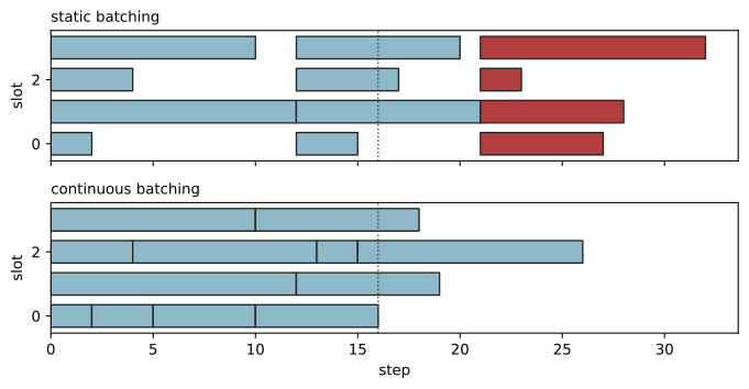
Continuous batching solves the compute holes. Variable length also strands memory: if every slot reserves a KV region sized for the longest possible sequence, short requests waste most of it. Memory becomes schedulable when the KV cache is paged. A request sees logical KV blocks in token order; a block table maps them to noncontiguous physical frames allocated only as tokens arrive (Kwon et al. 2023). We measure the waste directly, comparing a naive allocator that reserves max_len per sequence against a paged allocator that reserves whole blocks.
# @save
import math


def kv_fragmentation(lengths, block_size, max_len):
    """Compare KV memory reserved by contiguous vs paged allocation.

    A contiguous allocator reserves ``max_len`` tokens per sequence regardless
    of true length, stranding the difference; a paged allocator reserves whole
    ``block_size`` blocks, so its only waste is the partial final block of each
    sequence — bounded by less than one block per live sequence.

    Args:
        lengths: True token length of each live sequence.
        block_size: Tokens per KV block.
        max_len: Maximum sequence length the contiguous allocator reserves.

    Returns:
        A dict of tokens ``used``, tokens reserved by each allocator, each
        waste fraction, and the contiguous-over-paged reservation ratio.
    """
    used = sum(lengths)
    naive = len(lengths) * max_len
    paged = sum(math.ceil(length / block_size) * block_size for length in lengths)
    return {"used": used, "naive_reserved": naive, "paged_reserved": paged,
            "naive_waste": 1 - used / naive, "paged_waste": 1 - used / paged,
            "naive_over_paged": naive / paged}
We drive it with a realistic mix of live sequence lengths against a 256-token maximum and 16-token blocks.
live = [17, 5, 130, 44, 9, 88, 3, 61, 200, 12, 150, 7]
frag = kv_fragmentation(live, block_size=16, max_len=256)
print(f"tokens live: {frag['used']}")
print(f"contiguous reserves {frag['naive_reserved']} tokens "
      f"({frag['naive_waste']:.1%} wasted)")
print(f"paged      reserves {frag['paged_reserved']} tokens "
      f"({frag['paged_waste']:.1%} wasted)")
print(f"contiguous uses {frag['naive_over_paged']:.2f}x the KV memory")
tokens live: 726
contiguous reserves 3072 tokens (76.4% wasted)
paged reserves 832 tokens (12.7% wasted)
contiguous uses 3.69x the KV memoryFor a realistic length mix the contiguous allocator wastes 76% of its reserved KV and holds 3.7 times the memory the paged allocator needs. That saved memory is more concurrent sequences, which is more goodput at the same hardware. Paged blocks also make prefix sharing cheap: two sequences that begin with the same tokens point their block tables at the same physical frames for the shared prefix and get private frames only when they diverge — copy-on-write for KV. Figure 10.4 separates the logical order from the physical placement that makes this possible.
flowchart LR
    subgraph A["sequence A (logical)"]
        A0["prefix 0"] --> A1["prefix 1"] --> A2["private tail A"]
    end
    subgraph B["sequence B (logical)"]
        B0["prefix 0"] --> B1["prefix 1"] --> B2["private tail B"]
    end
    F7[("frame 7")]
    F9[("frame 9")]
    F4[("frame 4")]
    F2[("frame 2")]
    A0 --> F7
    B0 --> F7
    A1 --> F9
    B1 --> F9
    A2 -->|"copy on append"| F4
    B2 -->|"copy on append"| F2
10.3 Prefix caching pays off past a hit-rate threshold
An agent sends the same system instructions, tool schemas, and policy text on every turn. Recomputing their keys and values each time is pure waste — unless one request changed a timestamp near the front of the prompt, in which case the reuse silently misses. A different deployment gets frequent hits but accidentally lets two tenants share a prefix entry. Prefix caching is valuable only when identity, placement, and economics are all correct.
A prefix cache keeps KV blocks after their request finishes so a later request with the exact same token prefix and model state can skip that prefill. “Exact” is mechanical: semantically equal text with different token IDs is a miss, and equal token IDs computed under a different model, tokenizer, template, or adapter are not interchangeable. The cache key must cover every input that changes the KV values. We hash the token IDs and bind them to the revisions that produced them.
# @save
import hashlib
import json
from dataclasses import dataclass


@dataclass(frozen=True)
class CacheKey:
    """Identity fields that together make a cached prefix safe to reuse.

    Reuse is sound only when every input that could change the cached keys and
    values matches. The tenant field is policy, not mathematics: it keeps a hit
    from becoming a cross-tenant presence oracle even when the token IDs are
    identical.
    """

    tenant: str
    model_revision: str
    tokenizer_revision: str
    template_revision: str
    adapter_revision: str
    prefix_hash: str


def make_cache_key(tenant, token_ids, *, model="model-r1", tokenizer="tok-r1",
                   template="tmpl-r1", adapter="base"):
    """Hash exact token IDs with every state-changing revision into a CacheKey.

    Args:
        tenant: Trust domain the prefix belongs to.
        token_ids: The exact prefix token IDs; any difference is a miss.
        model, tokenizer, template, adapter: Revisions whose change would make
            the cached keys and values invalid for a new request.

    Returns:
        A ``CacheKey`` whose equality decides whether reuse is permitted.
    """
    digest = hashlib.sha256(json.dumps(token_ids, separators=(",", ":")).encode()).hexdigest()
    return CacheKey(tenant, model, tokenizer, template, adapter, digest[:16])
The same prefix reuses within a tenant and refuses to reuse across tenants.
prefix = list(range(45))
same = make_cache_key("tenant-a", prefix) == make_cache_key("tenant-a", prefix)
cross = make_cache_key("tenant-a", prefix) == make_cache_key("tenant-b", prefix)
print(f"same tenant, same prefix -> reuse: {same}")
print(f"different tenant, same prefix -> reuse: {cross}")
same tenant, same prefix -> reuse: True
different tenant, same prefix -> reuse: FalseIdentical prefixes reuse within a tenant and refuse to reuse across tenants — the isolation is in the key, not in a downstream check. Given a correct key, the remaining question is economic. Let C be the cost to recompute a prefix, C_w the cost to compute it once and write the cache entry, C_r the cost of one later read, and r the number of future reuses. Without caching the total is (1+r)C; with caching it is C_w + rC_r. When C_r < C, caching wins once
r > \frac{C_w - C}{C - C_r}. \tag{10.3}
Rather than a single break-even count, the more useful production view is the steady-state one: at hit rate h, each request pays C_r with probability h and C_w with probability {1-h}. We plot that effective cost against the baseline of always recomputing.
# @save
def cache_breakeven(compute, write, read):
    """Return the future reuses a cache write needs to beat recomputation.

    Implements @eq-ch10-breakeven. A read no cheaper than recomputation can
    never pay off on the critical path, so the function reports infinity.

    Args:
        compute: Cost to recompute the prefix.
        write: Cost to compute once and store the entry.
        read: Cost of one later cache read.

    Returns:
        The reuse count above which caching is cheaper, or ``inf``.
    """
    if read >= compute:
        return math.inf
    return max(0.0, (write - compute) / (compute - read))


def effective_cost(hit_rate, compute=1.0, write=1.25, read=0.10):
    """Average per-request prefix cost at a given cache hit rate.

    A hit pays ``read``; a miss pays ``write`` (compute plus store). The result
    is compared against the no-cache baseline of ``compute`` per request.

    Args:
        hit_rate: Fraction of requests served from cache.
        compute: No-cache recompute cost (the baseline).
        write: Miss cost: first compute plus writing the entry.
        read: Hit cost.

    Returns:
        The mean cost per request under caching.
    """
    return (1 - hit_rate) * write + hit_rate * read
We sweep the hit rate and find where the cached cost first drops below the recompute baseline.
hits = [i / 40 for i in range(41)]
costs = [effective_cost(h) for h in hits]
crossing = (1.25 - 1.0) / (1.25 - 0.10)          # cost(h) == baseline of 1.0
print(f"break-even reuse count (C=1, Cw=1.25, Cr=0.10): {cache_breakeven(1.0, 1.25, 0.10):.3f}")
print(f"caching beats recompute above hit rate ~{crossing:.2f}")
break-even reuse count (C=1, Cw=1.25, Cr=0.10): 0.278
caching beats recompute above hit rate ~0.22Below a hit rate of about 0.22 the write overhead on misses makes caching more expensive than recomputing; above it, reuse pays for the writes. Figure 10.5 draws the line. This is the same back-of-envelope cost arithmetic Chapter 33 systematizes for design interviews: a cache is only worth its bookkeeping once the hit rate clears its break-even.
Show the code that draws this figure
fig, ax = plt.subplots(figsize=(6.6, 3.4))
ax.plot(hits, costs, "-", color="#2a7f9e", label="cached (effective cost)")
ax.axhline(1.0, ls="--", color="#b13f3f", lw=1, label="no cache (baseline)")
ax.axvline(crossing, ls=":", color="#555", lw=1)
ax.set_xlabel("cache hit rate")
ax.set_ylabel("cost per request (units)")
ax.legend()
fig.tight_layout()
plt.show()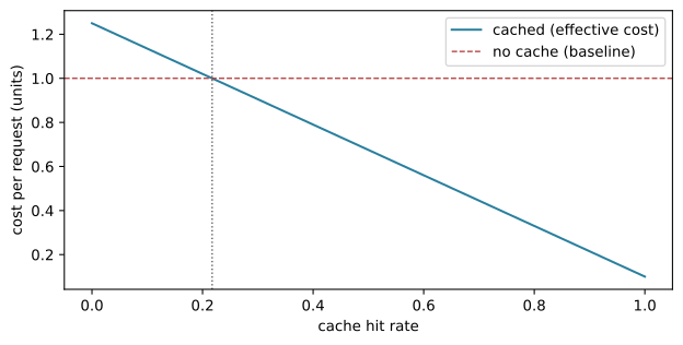
Eviction decides which entries survive under pressure. Approximate an entry’s value density as expected reuse probability times recomputation saved, divided by bytes retained — a 4000-token shared system prompt reused often is far denser than a one-off 200-token prompt, even though least-recently-used treats them alike. LRU is cheap when recency predicts reuse but fails on periodic jobs, scans, and large popular prefixes; size- and recomputation-aware scores protect the dense entries, and pinned prefixes need quotas. A radix tree over token IDs exposes shared paths so a router can prefer the replica holding the longest reusable prefix (Zheng et al. 2024), though always routing to the largest hit can create a hot replica — route on predicted completion, not raw hit length. Caller-side prompt ordering that maximizes reuse belongs to Chapter 13; the server hashes what it receives.
10.4 Speculative decoding trades compute for serial steps
Autoregressive decode waits for one target-model decision before it can build the next input. Speculative decoding hides that serial latency: a cheap draft model proposes several tokens at once, and the target verifies them in a single parallel pass, keeping the longest correct prefix (Leviathan et al. 2023). The verification is exact. A draft proposes token x from its distribution q; the target accepts it with probability a(x)=\min(1,\,p(x)/q(x)), and on rejection resamples from the normalized residual (p-q)_+. This correction reproduces the target distribution p exactly (Chen et al. 2023), and the expected one-token acceptance is
\sum_x q(x)\,a(x)=\sum_x \min(p(x),q(x))=1-\operatorname{TV}(p,q), \tag{10.4}
one minus the total-variation distance between draft and target. We implement one draw and verify the identity empirically over 40,000 samples.
# @save
import random


def categorical(probs, rng):
    """Draw one index from a categorical distribution with a seeded generator.

    Args:
        probs: A probability vector summing to one.
        rng: A ``random.Random`` supplying the uniform draw.

    Returns:
        The sampled index.
    """
    draw, total = rng.random(), 0.0
    for index, probability in enumerate(probs):
        total += probability
        if draw <= total:
            return index
    return len(probs) - 1


def speculative_draw(target, draft, rng):
    """Sample one exact target token through speculative accept/reject.

    Implements @eq-ch10-accept: a draft proposal is accepted with probability
    ``min(1, target/draft)``; on rejection the token is resampled from the
    positive residual ``(target - draft)+``. The emitted distribution equals
    ``target`` regardless of the draft's quality — the draft changes speed, not
    correctness.

    Args:
        target: The target model's next-token distribution.
        draft: The draft model's proposal distribution.
        rng: A ``random.Random`` for the proposal and accept draws.

    Returns:
        A ``(token, accepted)`` pair; ``accepted`` is False when the residual
        path was taken.
    """
    candidate = categorical(draft, rng)
    if rng.random() <= min(1.0, target[candidate] / draft[candidate]):
        return candidate, True
    residual = [max(p - q, 0.0) for p, q in zip(target, draft)]
    mass = sum(residual)
    return categorical([value / mass for value in residual], rng), False
We draw 40,000 samples and check the empirical acceptance and the emitted distribution against the target.
target, draft = [0.52, 0.28, 0.15, 0.05], [0.42, 0.32, 0.18, 0.08]
counts, accepts, rng = [0] * 4, 0, random.Random(731)
for _ in range(40_000):
    token, accepted = speculative_draw(target, draft, rng)
    counts[token] += 1; accepts += accepted
empirical = [c / 40_000 for c in counts]
alpha = sum(min(p, q) for p, q in zip(target, draft))
tv = sum(abs(a - b) for a, b in zip(empirical, target)) / 2
print(f"predicted acceptance 1-TV: {alpha:.4f}   empirical accept rate: {accepts/40_000:.4f}")
print(f"total variation of emitted vs target: {tv:.5f}  (exact => ~0)")
predicted acceptance 1-TV: 0.9000 empirical accept rate: 0.9008
total variation of emitted vs target: 0.00365 (exact => ~0)The empirical acceptance matches {1-\text{TV}=0.90} and the emitted distribution reproduces the target to within sampling noise: exactness holds. But exactness is not speedup. For a draft block of \gamma proposed tokens with per-token acceptance \alpha, the expected number accepted before the first rejection is the geometric sum
E(\alpha,\gamma)=\sum_{k=0}^{\gamma}\alpha^{k}=\frac{1-\alpha^{\gamma+1}}{1-\alpha}. \tag{10.5}
Speedup is those accepted tokens divided by the added work: one target verification plus \gamma draft steps, each costing some fraction of a target step. When the fleet is idle the draft is nearly free; under contention the draft competes for the same accelerator and its per-token cost rises.
# @save
def expected_accepted_tokens(alpha, block):
    """Expected tokens accepted per verification for a draft block (@eq-ch10-spectokens).

    Args:
        alpha: Per-token acceptance probability (``1 - TV`` of @eq-ch10-accept).
        block: Number of tokens the draft proposes before verification.

    Returns:
        The geometric-sum expectation ``(1 - alpha**(block+1)) / (1 - alpha)``.
    """
    return sum(alpha ** k for k in range(block + 1))


def speculative_speedup(alpha, block, draft_cost):
    """Speedup of speculative decoding relative to plain autoregressive decode.

    Divides expected accepted tokens by the added work of one verification plus
    ``block`` draft steps at ``draft_cost`` each. A cheap draft (idle fleet)
    gives a large speedup; an expensive draft (saturated fleet) can push the
    ratio below one, so an isolated latency win becomes a goodput loss.

    Args:
        alpha: Per-token acceptance probability.
        block: Draft block length.
        draft_cost: Cost of one draft token as a fraction of a target step.

    Returns:
        The speedup factor; below 1.0 means speculation is a net loss.
    """
    return expected_accepted_tokens(alpha, block) / (1 + block * draft_cost)
We compare the idle-fleet and saturated-fleet regimes across a range of acceptance rates.
for a in (0.6, 0.75, 0.85, 0.9, 0.95):
    low = speculative_speedup(a, 4, draft_cost=0.05)
    saturated = speculative_speedup(a, 4, draft_cost=0.85)
    print(f"acceptance {a:.2f}: idle-fleet speedup {low:.2f}x   "
          f"saturated-fleet speedup {saturated:.2f}x")
acceptance 0.60: idle-fleet speedup 1.92x saturated-fleet speedup 0.52x
acceptance 0.75: idle-fleet speedup 2.54x saturated-fleet speedup 0.69x
acceptance 0.85: idle-fleet speedup 3.09x saturated-fleet speedup 0.84x
acceptance 0.90: idle-fleet speedup 3.41x saturated-fleet speedup 0.93x
acceptance 0.95: idle-fleet speedup 3.77x saturated-fleet speedup 1.03xAt acceptance 0.90 with a draft block of four, an idle fleet sees a 3.4x speedup; a saturated fleet sees 0.93x — a net loss, because the draft’s extra work now steals from the target. Only at very high acceptance does speculation stay positive under contention. Figure 10.6 shows the two regimes and where the saturated curve crosses one.
Show the code that draws this figure
grid = [a / 100 for a in range(40, 98)]
fig, ax = plt.subplots(figsize=(6.6, 3.6))
ax.plot(grid, [speculative_speedup(a, 4, 0.05) for a in grid], "-", color="#2a7f9e", label="idle fleet (draft cost 0.05)")
ax.plot(grid, [speculative_speedup(a, 4, 0.85) for a in grid], "-", color="#b13f3f", label="saturated fleet (draft cost 0.85)")
ax.axhline(1.0, ls="--", color="#555", lw=1)
ax.set_xlabel("draft acceptance rate")
ax.set_ylabel("speedup vs plain decode")
ax.legend()
fig.tight_layout()
plt.show()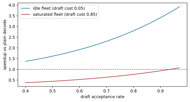
10.5 Quantization is a validation problem
A four-bit checkpoint occupies less storage than its parent yet serves fewer requests per second because its engine dequantizes through an unfused kernel, and an important tool-selection task regresses even though perplexity barely moves. “Four bit” described storage, not the numerical and execution contract. Quantization approximates high-precision values with a smaller representation, and a recipe is specified along independent axes: what is quantized (weights, activations, KV, communication buffers), the numerical family and width, the scale granularity (tensor, channel, group, block), when scales are chosen (static or per-input), the accumulator precision, and the kernel and hardware support. W4A16 means four-bit weights and sixteen-bit activations; weight-only recipes target decode’s weight-bandwidth bottleneck.
For symmetric integer quantization of a tensor row x with b bits, choose a per-row scale s = \max_i|x_i| / Q with Q=2^{b-1}-1, then
q_i=\operatorname{clip}(\operatorname{round}(x_i/s),\,-Q,\,Q),\qquad \hat{x}_i=s\,q_i. \tag{10.6}
We apply this to a real model: the tiny GPT trained in Chapter 2. First we retrain a small one on a structured toy corpus so its next-token accuracy is measurable, then we quantize its weights and read the damage honestly.
import sys
sys.path.insert(0, "code/ch02")
import _generated as ch02              # the TinyGPT we built in Chapter 2
import torch

corpus_rng = random.Random(7)
nouns = ["apple", "book", "cup", "lamp", "chair", "phone", "shoe", "clock"]
colors = ["red", "blue", "green", "gray"]
corpus = " ".join(f"the {corpus_rng.choice(colors)} {corpus_rng.choice(nouns)} "
                  f"has value {corpus_rng.randint(1, 9)} ." for _ in range(700))
tokenizer = ch02.BytePairTokenizer.train(corpus, vocab_size=288)
ids = torch.tensor(tokenizer.encode(corpus), dtype=torch.long)
config = ch02.GPTConfig(vocab_size=tokenizer.vocab_size, block_size=48,
                        d_model=64, n_heads=4, n_layers=2)
print(f"corpus {len(corpus)} chars -> {ids.numel()} tokens, vocab {tokenizer.vocab_size}")
corpus 19831 chars -> 4633 tokens, vocab 288We train for 250 steps — enough for the toy model to learn the corpus’s rigid structure — and record its held-out next-token accuracy in full precision.
torch.manual_seed(0)
model = ch02.TinyGPT(config)
optimizer = torch.optim.AdamW(model.parameters(), lr=3e-3)
batches = torch.Generator().manual_seed(0)
split = int(0.9 * ids.numel())
train_ids, val_ids = ids[:split], ids[split:]
model.train()
for step in range(250):
    xb, yb = ch02.next_token_batch(train_ids, config.block_size, 32, batches)
    _, loss, _ = model(xb, yb)
    optimizer.zero_grad(); loss.backward(); optimizer.step()
model.eval()
with torch.inference_mode():
    xb, yb = ch02.next_token_batch(val_ids, config.block_size, 96, torch.Generator().manual_seed(1))
    reference_logits, _, _ = model(xb)
    reference_acc = (reference_logits.argmax(-1) == yb).float().mean().item()
print(f"trained loss {loss.item():.3f}  held-out next-token accuracy {reference_acc:.3f}")
trained loss 0.847 held-out next-token accuracy 0.596Now the quantizer. We quantize every two-dimensional weight per row with Equation 10.6, load the result into a fresh model, and compare. Because the represented values are the dequantized \hat{x}, this measures exactly the numerical error a weight-only integer kernel would incur.
# @save
import torch


def quantize_tensor(weight, bits):
    """Symmetric per-row integer quantization of a 2-D weight (@eq-ch10-symquant).

    Each row gets its own scale from its largest magnitude, so an outlier in one
    row cannot inflate the step size of another. The returned tensor holds the
    dequantized values a real integer kernel would compute against.

    Args:
        weight: A 2-D floating-point weight tensor.
        bits: Integer width; the signed bound is ``2**(bits-1) - 1``.

    Returns:
        The dequantized tensor, same shape and dtype as ``weight``.
    """
    qmax = 2 ** (bits - 1) - 1
    scale = weight.abs().amax(dim=-1, keepdim=True).clamp_min(1e-12) / qmax
    return torch.clamp(torch.round(weight / scale), -qmax, qmax) * scale


def model_storage(model, bits):
    """Return (fp32_bytes, quantized_bytes) counting each weight once.

    Quantized 2-D weights cost ``bits/8`` bytes plus a 16-bit per-row scale;
    everything else stays 32-bit. Tied weights are deduped by identity so a
    shared embedding and LM head are not charged twice.

    Args:
        model: The module to size.
        bits: Integer width applied to 2-D float weights.

    Returns:
        A ``(fp32_bytes, quantized_bytes)`` tuple.
    """
    seen, fp32, quant = set(), 0, 0
    for _, p in model.named_parameters():
        if id(p) in seen:
            continue
        seen.add(id(p))
        fp32 += p.numel() * 4
        if p.dim() == 2 and p.dtype.is_floating_point:
            quant += p.numel() * bits // 8 + p.shape[0] * 2
        else:
            quant += p.numel() * 4
    return fp32, quant
We size the model, then run the int8 and int4 ladder: quantize every weight, reload, and read accuracy, KL divergence from the full-precision distribution, and maximum logit drift.
reference_probs = reference_logits.softmax(-1)
fp32_bytes, _ = model_storage(model, 8)
print(f"full precision: {fp32_bytes} bytes, accuracy {reference_acc:.3f}")
for bits in (8, 4):
    quantized = ch02.TinyGPT(config)
    quantized.load_state_dict({name: (quantize_tensor(p, bits)
                                      if p.dim() == 2 and p.dtype.is_floating_point else p.clone())
                               for name, p in model.state_dict().items()})
    quantized.eval()
    with torch.inference_mode():
        q_logits, _, _ = quantized(xb)
        q_acc = (q_logits.argmax(-1) == yb).float().mean().item()
        q_probs = q_logits.softmax(-1)
        kl = (reference_probs * (reference_probs.clamp_min(1e-9).log()
              - q_probs.clamp_min(1e-9).log())).sum(-1).mean().item()
        drift = (reference_logits - q_logits).abs().max().item()
    _, q_bytes = model_storage(model, bits)
    print(f"int{bits}: accuracy {q_acc:.3f}  KL {kl:.4f}  max logit drift {drift:.3f}  "
          f"{fp32_bytes / q_bytes:.2f}x smaller")
full precision: 481280 bytes, accuracy 0.596
int8: accuracy 0.595 KL 0.0000 max logit drift 0.112 3.86x smaller
int4: accuracy 0.601 KL 0.0026 max logit drift 1.317 7.42x smallerPer-row int8 is nearly lossless at this scale: accuracy is unchanged, the KL divergence from the full-precision distribution is essentially zero, and the model is 3.9 times smaller. Int4 is where “validation problem” earns its name — the same model loses accuracy and its logits drift by several units, all from halving the width again. The lesson is not that int8 is safe and int4 is not in general; it is that only measurement tells you, and the metric that moved (a tool-selection task) may not be the one you watched (perplexity).
Outliers are why finer granularity helps. A single large value in a block forces a coarse scale on all its neighbors. We show this with a 256-value vector carrying two planted outliers, quantized to four bits at three block sizes.
# @save
def quantize_blockwise(values, bits, block_size):
    """Symmetric integer quantization applied independently to each block.

    A smaller block gives each local range its own scale, so a distant outlier
    can no longer coarsen a whole tensor's step size — at the cost of storing
    one more scale per block (the effective-width overhead ``b_s / g``).

    Args:
        values: The sequence to quantize.
        bits: Integer width.
        block_size: Values sharing one scale.

    Returns:
        A ``(reconstructed, rmse)`` pair.
    """
    qmax, restored = 2 ** (bits - 1) - 1, []
    for base in range(0, len(values), block_size):
        block = values[base:base + block_size]
        scale = max(abs(v) for v in block) / qmax or 1.0
        restored.extend(max(-qmax, min(qmax, round(v / scale))) * scale for v in block)
    rmse = math.sqrt(sum((a - b) ** 2 for a, b in zip(values, restored)) / len(values))
    return restored, rmse
We build a 256-value signal, plant two outliers, and quantize it to four bits at three block sizes.
signal = [2 * math.sin(i / 11) + 0.3 * math.cos(i / 3) for i in range(256)]
signal[47], signal[181] = 38.0, -29.0
blocks = [(bs, quantize_blockwise(signal, 4, bs)[1], 4 + 16 / bs) for bs in (16, 64, 256)]
for bs, rmse, eff in blocks:
    print(f"block {bs:>3}: RMSE {rmse:.3f}  effective bits/value {eff:.3f}")
block 16: RMSE 0.455 effective bits/value 5.000
block 64: RMSE 0.978 effective bits/value 4.250
block 256: RMSE 1.415 effective bits/value 4.062At block 16 each outlier contaminates only fifteen neighbors and the RMSE is a third of the whole-tensor case, but the stored scales push the effective width to 5.0 bits — “four bit” is really 4.06, 4.25, or 5.0 depending on granularity. Figure 10.7 makes the trade visible. Activation-aware recipes attack the same outliers differently: SmoothQuant migrates difficulty from activations into weights with the identity XW=(XD^{-1})(DW) for a diagonal D, rescaling activations into a friendlier range while folding the inverse into offline-calibrated weights (Xiao et al. 2023); weight-only methods like GPTQ and AWQ instead protect the salient channels (Frantar et al. 2023; Lin et al. 2024). The algebra is exact; the quantization is where the approximation enters, so calibration data and shapes must match deployment.
Show the code that draws this figure
fig, (ax1, ax2) = plt.subplots(1, 2, figsize=(7.6, 3.2))
ax1.plot(signal, color="#333", lw=0.8)
ax1.set_title("signal with 2 outliers", fontsize=10)
ax1.set_xlabel("index"); ax1.set_ylabel("value")
sizes = [b[0] for b in blocks]
ax2.plot(sizes, [b[1] for b in blocks], "o-", color="#b13f3f")
for bs, rmse, eff in blocks:
    ax2.annotate(f"{eff:.2f} bits", (bs, rmse), textcoords="offset points", xytext=(6, 6), fontsize=8)
ax2.set_title("4-bit error vs block size", fontsize=10)
ax2.set_xlabel("block size (values)"); ax2.set_ylabel("RMSE")
fig.tight_layout()
plt.show()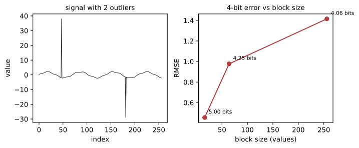
10.6 Constrained decoding masks the tokens a grammar forbids
Callers want structured output — JSON that parses, an enum value, a schema-valid object. Constrained decoding guarantees it by construction: at each step the runtime advances a parser, computes which tokens can continue a valid parse, masks the rest to probability zero, renormalizes, and samples. A finite-state machine covers regular constraints (fixed choices, lexical patterns); a context-free grammar adds a stack for nested structures (Dong et al. 2024). The mechanics are a mask and a renormalization; if illegal tokens hold mass m, masking removes m and the survivors are rescaled to sum to one.
# @save
def constrained_distribution(probs, allowed):
    """Mask disallowed tokens to zero and renormalize the survivors.

    This is exact for the *constrained* distribution: it is the target
    distribution conditioned on the grammar's allowed set. The reported removed
    mass is how strongly the model wanted a token the grammar forbids.

    Args:
        probs: The model's next-token distribution.
        allowed: Indices the grammar permits at this parser state.

    Returns:
        A dict with the renormalized ``distribution`` and the ``removed_mass``.

    Raises:
        ValueError: If the allowed set holds no probability (unsatisfiable).
    """
    kept = sum(probs[i] for i in allowed)
    if kept == 0:
        raise ValueError("grammar admits no token here")
    return {"distribution": [p / kept if i in allowed else 0.0 for i, p in enumerate(probs)],
            "removed_mass": 1 - kept}
A toy three-token distribution shows the mechanics: forbid one token and the survivors renormalize.
toy = constrained_distribution([0.60, 0.25, 0.15], {1, 2})
print(f"toy: removed {toy['removed_mass']:.2f} of the mass, "
      f"renormalized sums to {sum(toy['distribution']):.3f}")
toy: removed 0.60 of the mass, renormalized sums to 1.000The toy vector removes 0.60 of the mass and rebalances the rest. The genuinely hard part is not the mask but tokenization: the parser reasons about characters, while the model emits tokens, and one token can span several characters, split a delimiter, or cross a grammar transition. We see this directly in the tokenizer we just trained.
sample = "the red cup has value 8 ."
pieces = [tokenizer.token_bytes[i].decode("latin-1") for i in tokenizer.encode(sample)]
print(f"{len(sample)} characters -> {len(pieces)} tokens:")
print(pieces)
25 characters -> 8 tokens:
['the ', 're', 'd', ' c', 'u', 'p has value ', '8', ' .']A single token, "p has value ", bundles the tail of one word with three whole words — a “must emit a digit next” rule cannot be enforced by picking “digit tokens” alone, because the model’s natural continuations hide digits inside larger tokens. Now we apply a real grammar mask to the real model. After the prompt the red apple has value, the grammar requires a bare digit; we intersect that with the model’s actual next-token logits.
digit_tokens = [i for i in range(tokenizer.vocab_size)
                if tokenizer.token_bytes[i].decode("latin-1").isdigit()]
context = torch.tensor([tokenizer.encode("the red apple has value ")])
with torch.inference_mode():
    logits, _, _ = model(context)
distribution = logits[0, -1].softmax(-1).tolist()
free_top = tokenizer.token_bytes[max(range(len(distribution)),
                                     key=distribution.__getitem__)].decode("latin-1")
masked = constrained_distribution(distribution, set(digit_tokens))
con_top = tokenizer.token_bytes[max(range(len(masked["distribution"])),
                                    key=masked["distribution"].__getitem__)].decode("latin-1")
print(f"{len(digit_tokens)} digit tokens in vocab")
print(f"unconstrained top token: {free_top!r}   removed mass under grammar: {masked['removed_mass']:.3f}")
print(f"constrained top token: {con_top!r}")
13 digit tokens in vocab
unconstrained top token: '1' removed mass under grammar: 0.016
constrained top token: '1'Here the trained model already learned that a digit follows value, so the grammar removes almost none of the mass and picks the same token — when the model respects the grammar, the constraint is nearly free. Point the same mask at a context where the model wants prose and the removed mass jumps toward one, and the constrained sample is drawn from the rare surviving tokens. Figure 10.8 traces the pipeline, including the tokenization boundary that makes it subtle.
flowchart LR
    P["parser state"] --> A["allowed byte-strings"]
    A --> X["intersect with vocab<br/>(a token may cross the boundary)"]
    X --> M["mask logits -> -inf"]
    M --> N["renormalize survivors"]
    N --> S(["sample a valid token"])
    S -->|"advance parser"| P
A grammar guarantees syntax, not truth or authorization — Chapter 17 and Chapter 24 validate values and authorize effects. And because format restrictions can crowd out reasoning, a common design separates a long deliberation from a small validated final object.
10.7 Disaggregation, eviction, and the memory-bandwidth split
A decode stream produces a token every few milliseconds until a long prompt enters the same worker. That prompt’s prefill turns one scheduler iteration into a large compute job, and every active stream stalls behind it. Two controls address this. Chunked prefill slices a long prompt into bounded chunks interleaved with decode, capping the stall at the cost of some overhead (Agrawal et al. 2024). Prefill/decode disaggregation goes further: a prefill worker materializes the KV state and hands it to a separate decode worker, so the two phases run on hardware sized for their different bottlenecks — prefill is compute-bound, decode is memory-bandwidth- and KV-capacity-bound (Zhong et al. 2024; Patel et al. 2024).
The split is not free. Removing interference recovers latency \Delta I and specialization gains \Delta S, but adds KV-transfer time T_{KV}, routing and coordination T_R, queue imbalance T_Q, and expected failure cost T_F. Disaggregate only when
\Delta I+\Delta S > T_{KV}+T_R+T_Q+T_F, \tag{10.7}
and note that T_{KV}\ge M_{KV}/B_{\text{eff}}: moving more KV bytes across a slower path can erase the gain. We apply the inequality to two fixtures.
# @save
def disaggregation_decision(kv_gib, interference_saved_ms, bandwidth_gibps=200.0,
                            coordination_ms=2.8):
    """Decide whether phase disaggregation beats a co-located worker (@eq-ch10-disagg).

    Charges KV transfer as ``kv_gib / bandwidth`` plus fixed coordination, and
    compares that overhead against the interference latency removing prefill
    from the decode path recovers. Longer prompts save more interference but
    also move more KV, so the decision can flip with prompt size.

    Args:
        kv_gib: KV state to transfer between pools, in GiB.
        interference_saved_ms: Latency recovered by removing co-location.
        bandwidth_gibps: Effective transfer bandwidth, GiB/s.
        coordination_ms: Routing, handshake, and expected-retry overhead.

    Returns:
        A dict with the transfer and total overhead, and the ``disaggregate``
        verdict.
    """
    transfer_ms = kv_gib / bandwidth_gibps * 1000
    overhead_ms = transfer_ms + coordination_ms
    return {"kv_gib": kv_gib, "transfer_ms": transfer_ms, "overhead_ms": overhead_ms,
            "interference_saved_ms": interference_saved_ms,
            "disaggregate": interference_saved_ms > overhead_ms}
We apply it to a small-KV short prompt and a large-KV long prompt.
for name, kv, saved in (("short prompt", 0.25, 3.0), ("long prompt", 4.0, 35.0)):
    d = disaggregation_decision(kv, saved)
    print(f"{name}: saves {saved} ms, pays {d['overhead_ms']:.2f} ms "
          f"-> disaggregate: {d['disaggregate']}")
short prompt: saves 3.0 ms, pays 4.05 ms -> disaggregate: False
long prompt: saves 35.0 ms, pays 22.80 ms -> disaggregate: TrueThe short prompt saves 3 ms of interference but pays 4 ms to move its small KV plus coordinate — a loss. The long prompt saves 35 ms and pays 23 ms even with a larger transfer — a win. A static prefill/decode ratio fails when traffic composition shifts, so controllers reassign roles or route short prompts through co-located workers. Figure 10.9 shows where the coordination and transfer cost lands.
sequenceDiagram
    participant C as Caller
    participant R as SLO-aware router
    participant P as Prefill pool
    participant K as KV transport
    participant D as Decode pool
    C->>R: prompt, deadline
    R->>P: admit prefill
    P->>K: publish KV + identity
    K->>D: transfer authorized KV
    D-->>R: ready after KV validation
    D-->>C: stream tokens
    alt deadline expiry
        R-->>P: cancel prefill
        R-->>D: release frames
    end
The same memory-pressure logic drives KV eviction and compression: under load the server must free frames, and the value-density score from Section 10.3 decides what to drop — evict the cheap-to-recompute, rarely-reused entries first, and consider low-precision KV (the quantization ladder above, now applied to the cache) before discarding state that a long context will need again. Long-context serving is this problem at scale: KV grows linearly with tokens (Chapter 3), so ring or chunked-context schemes and aggressive eviction are how a fixed KV pool serves sequences longer than it could hold at full precision.
10.8 Multi-tenant serving shares more than weights
When one model does not fit or one replica cannot meet demand, “use more GPUs” hides the real choice. Parallel strategies move different data at different frequencies, and serving magnifies their cost because decode runs many small latency-sensitive steps rather than a few large training batches.
| Strategy | What is divided | Serving advantage | Dominant serving risk |
|---|---|---|---|
| Data-parallel replicas | requests, full model copies | independent scaling and failure domains | load and prefix-cache imbalance |
| Tensor parallelism | tensors within each layer | makes a layer fit; pools device bandwidth | collective on every layer and decode step |
| Pipeline parallelism | consecutive layer groups | crosses nodes with fewer, larger transfers | pipeline bubbles and per-request latency |
| Expert parallelism | mixture-of-experts weights | distributes a sparse model’s expert memory | token all-to-all and hot experts |
Mixture-of-experts serving is the case where these interact hardest: expert parallelism spreads expert weights across devices, but sparse activation lowers arithmetic, not the all-to-all communication or the expert storage, and a hot expert sets the batch’s step time. Benchmark the actual topology; an oversubscribed interconnect erases the arithmetic saving.
Multi-LoRA tenancy shares the expensive base xW while applying per-tenant low-rank xAB terms on the fly, so one replica serves thousands of adapters without a merged weight matrix per tenant; grouped kernels batch the heterogeneous adapter terms (Sheng et al. 2024). But sharing a base model, process, accelerator, or cache widens the security boundary, and the sharpest serving-specific risk is a timing side channel: a cache hit is fast and a miss is slow, so if the cache key omits the tenant, one tenant can detect another’s prefix by timing a lookup. We demonstrate the leak and its fix.
# @save
def shared_prefix_leak(include_tenant):
    """Show whether a prefix cache leaks cross-tenant presence by hit timing.

    Tenant B warms a prefix; tenant A then probes the same token IDs. A hit is
    cheap and a miss is expensive, so if the cache key omits the tenant, tenant
    A's fast probe reveals that tenant B used the prefix — a presence oracle.
    Binding the tenant into the key (as ``make_cache_key`` does) turns the probe
    into a miss and closes the channel.

    Args:
        include_tenant: Whether the cache key includes the tenant identity.

    Returns:
        A dict with the probe's ``hit`` result and whether presence ``leaked``.
    """
    prefix = list(range(60))
    cache = {}

    def key(tenant):
        return (tenant, tuple(prefix)) if include_tenant else tuple(prefix)

    cache[key("tenant-b")] = "warm"                 # tenant B warms the prefix
    hit = key("tenant-a") in cache                  # tenant A probes it
    return {"probe_hit": hit, "leaked_presence": hit}
We run both key policies and see which one lets tenant A detect tenant B’s prefix.
for policy in (False, True):
    result = shared_prefix_leak(include_tenant=policy)
    label = "tenant-scoped key" if policy else "prefix-only key"
    print(f"{label:>18}: probe hit {result['probe_hit']!s:>5}  "
          f"leaks presence: {result['leaked_presence']}")
prefix-only key: probe hit True leaks presence: True
tenant-scoped key: probe hit False leaks presence: FalseWith a prefix-only key, tenant A’s probe hits tenant B’s entry and the timing reveals presence; the tenant-scoped key makes it a miss and closes the channel. This is one demonstrated control; the full threat model — residual KV recovery from unscrubbed device memory (Sorensen and Khlaaf 2024), adapter integrity and authorization, cache zeroization on cancellation and crash, encrypted remote KV, and accelerator attestation — belongs to Chapter 24, which serving must implement but does not own. The minimum serving contract is: tenant-scoped keys over every revision, quotas on KV bytes and adapters, and explicit zeroization on release.
To measure a real endpoint against these mechanics, an OpenAI-compatible route gives interface portability. The seam below times first content and inter-event gaps; it is a measurement probe, not a load generator, and it is the one cell in this chapter that needs a network.
import time, urllib.request

def profile_endpoint(base_url, model, prompt, max_tokens=64):
    """Time first-content latency and stream gaps for an OpenAI-compatible route."""
    body = json.dumps({"model": model, "messages": [{"role": "user", "content": prompt}],
                       "max_tokens": max_tokens, "temperature": 0, "stream": True}).encode()
    request = urllib.request.Request(base_url.rstrip("/") + "/v1/chat/completions",
                                     data=body, headers={"Content-Type": "application/json"})
    start, first = time.perf_counter(), None
    with urllib.request.urlopen(request) as response:
        for line in response:
            if line.startswith(b"data:") and b"content" in line and first is None:
                first = time.perf_counter() - start
    return {"ttft_seconds": first}
10.9 Production test-time compute needs a budget
A reasoning model improves a hard planning task when it thinks longer, so a service enables the highest reasoning tier for every request. Simple requests now hold decode slots and KV frames for hundreds of extra tokens; queueing pushes hard requests past their deadlines; total successful work falls. More compute improved isolated accuracy while reducing production goodput. Chapter 8 treated test-time compute as search and verification; in serving, a reasoning budget is a reservation — tokens, effort tier, deadline, candidates — that must be priced against its cost. A budget policy continues spending only while marginal value exceeds marginal system cost:
\Delta p\,V > \Delta n\,c_n + \Delta h\,c_h + D, \tag{10.8}
where \Delta p is the gain in task success, V its value, \Delta n the extra tokens at unit cost c_n, \Delta h the added KV holding time at capacity shadow price c_h, and D the harm from delay. The shadow price c_h rises near the goodput knee, so the right budget is load-aware. We measure the value side with a toy reasoner whose accuracy follows the coverage law of Chapter 8: more thinking means more sampled candidates and a higher chance of hitting the answer — until an overthinking tail, where the model second-guesses a found answer.
# @save
def budget_forcing_sweep(budgets, trials=4000, candidates=40, tokens_per_thought=8,
                         derail_rate=0.0016, seed=0):
    """Sweep a toy reasoner's accuracy against a thinking-token budget.

    Each thought samples one candidate; coverage rises as the budget buys more
    samples (the @sec-ch08 coverage law). Past a point an overthinking term
    switches away from a found answer with probability growing in the budget, so
    accuracy saturates and then declines while tokens keep accruing — the shape
    that forces @eq-ch10-budget to stop early. Budget forcing is the truncation
    at each swept budget; the curve is illustrative, not a model measurement.

    Args:
        budgets: Thinking-token budgets to sweep.
        trials: Independent tasks per budget.
        candidates: Answer-space size; per-sample hit probability is ``1/candidates``.
        tokens_per_thought: Tokens each sampled candidate costs.
        derail_rate: Overthinking rate; derail probability is ``1 - exp(-rate*budget)``.
        seed: Seed for the sampling.

    Returns:
        One dict per budget with ``accuracy`` and accuracy ``per_1k`` tokens.
    """
    rng = random.Random(seed)
    rows = []
    for budget in budgets:
        samples = max(1, budget // tokens_per_thought)
        correct = 0
        for _ in range(trials):
            found = any(rng.random() < 1.0 / candidates for _ in range(samples))
            if found and rng.random() < 1 - math.exp(-derail_rate * budget):
                found = False
            correct += found
        accuracy = correct / trials
        rows.append({"budget": budget, "accuracy": accuracy,
                     "per_1k": accuracy * 1000 / budget})
    return rows
We sweep a range of budgets and print accuracy and its per-token efficiency.
sweep = budget_forcing_sweep([32, 64, 128, 256, 384, 512, 768])
print(f"{'budget':>7} {'accuracy':>9} {'acc/1k tokens':>14}")
for row in sweep:
    print(f"{row['budget']:>7} {row['accuracy']:>9.3f} {row['per_1k']:>14.3f}")
budget accuracy acc/1k tokens
32 0.102 3.172
64 0.160 2.500
128 0.268 2.096
256 0.379 1.479
384 0.386 1.005
512 0.362 0.707
768 0.279 0.363Accuracy climbs from 0.10 at 32 tokens to a peak near 0.39 at 384, then declines as overthinking sets in, while accuracy per thousand tokens falls monotonically the whole way. The marginal-value stop is well before the peak: the jump from 256 to 384 tokens buys almost nothing and 384 to 512 is negative. Figure 10.10 marks where the budget should stop.
Show the code that draws this figure
budgets = [r["budget"] for r in sweep]
fig, ax = plt.subplots(figsize=(6.6, 3.6))
ax.plot(budgets, [r["accuracy"] for r in sweep], "o-", color="#b13f3f", label="accuracy")
peak = max(sweep, key=lambda r: r["accuracy"])["budget"]
ax.axvline(peak, ls=":", color="#555", lw=1)
ax.set_xlabel("thinking-token budget"); ax.set_ylabel("accuracy", color="#b13f3f")
twin = ax.twinx()
twin.plot(budgets, [r["per_1k"] for r in sweep], "s--", color="#2a7f9e", label="accuracy / 1k tokens")
twin.set_ylabel("accuracy per 1k tokens", color="#2a7f9e")
fig.tight_layout()
plt.show()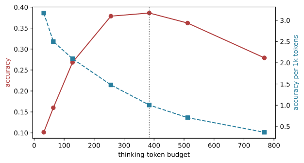
Inference-time budget forcing enforces exactly this stop by truncating or extending a trace; s1 studied it as an experimental control (Muennighoff et al. 2025), and training-time length control teaches requested lengths directly (Aggarwal and Welleck 2025). Neither guarantees monotonic quality — truncation can cut a solution, continuation can overthink — so a served policy starts cheap, escalates only when a verifier predicts value, and enforces a hard deadline. Hidden reasoning still consumes decode steps and KV even when only a summary returns, so telemetry should track budgets, timings, and verifier outcomes rather than logging private chains of thought, whose faithfulness Chapter 25 owns.
10.10 Landscape 2026: local inference and the hardware floor
Verified on 2026-07-19. The mechanisms above are engine-independent; the products that implement them, and the hardware they target, move quarterly.
- Local inference.
llama.cppand its GGUF k-quant formats serve quantized models on CPU and consumer GPUs; MLX targets Apple silicon’s unified memory; Ollama and LM Studio package local serving. Unified-memory laptops now hold models that needed a data-center GPU in 2023; the binding constraint is memory bandwidth, not FLOPs. - Quantization formats. The OCP MX specification defines MXFP4 (an 8-bit scale per 32 FP4 values, ~4.25 bits/value); NVIDIA NVFP4 uses an FP8 scale per 16 values. Nominal width predicts neither quality nor speed without kernel support.
- Serving engines. vLLM, SGLang, and TensorRT-LLM implement paging, prefix caching, speculation, and disaggregation to different depths; the combination you need may fall on an unfused path. Inspect the pinned feature matrix, not the headline benchmark.
- Provider reasoning surfaces. Hosted reasoning-effort controls, their defaults, visibility, cache interaction, and prices vary by provider and change often; exposed reasoning is not evidence of faithfulness.
Verify live: engine feature-combination support; quantization scale layouts and hardware requirements; prefix-cache isolation and hash inputs; speculative and disaggregated-KV protocols; provider reasoning-effort names, usage accounting, and caching; local-server backends; versions, licenses, and security advisories.
10.11 Summary
Serving optimizes goodput — completions that meet every SLO — not raw throughput, and the two diverge past a load knee we drew by simulation. Continuous batching fills the slots a fixed batch idles; paged KV reclaims the memory a contiguous cache strands and enables prefix sharing. Prefix caching pays off only above a hit-rate break-even. Speculative decoding is exact but speeds a request up only when the draft is cheap. Quantization is a validation problem: per-row int8 barely moved our tiny GPT while int4 drifted. Constrained decoding masks logits to a grammar across a tricky tokenization boundary. Disaggregation, eviction, tenancy isolation, and reasoning budgets each trade one resource for another; Chapter 11 serves customized variants of these models.
10.12 Exercises
Move the goodput knee. Using
sweep_load, sweepslotsandmean_serviceas well asrate. (a) Confirm the capacityslots / mean_servicepredicts where throughput saturates. (b) Find the arrival rate at which goodput peaks for two differentttft_slovalues and explain why a tighter SLO moves the knee left. (c) Add a second SLO on completion time and show a workload where the two-SLO goodput is far below either single-SLO rate.Verify the scheduler by hand. For the twelve-request burst, redraw the four slots for all 26 continuous-batching steps and recompute each start, finish, and the TTFT/TPOT test. Then permute the request order to raise static-batch utilization, and state which queueing assumption your permutation quietly violates.
Break speculative speedup without breaking exactness. With
speculative_speedup, sweep block length, acceptance, and draft cost. Predict the acceptance at which the saturated-fleet curve crosses 1.0 before running it, then add a statistical test that the emitted distribution still equals the target — showing a configuration whose isolated latency improves while saturated goodput falls.Push the quantization until it breaks. Extend
quantize_tensorto int3 and int2 and re-run the ladder on the trained model. Report accuracy, KL, and max logit drift at each width, and identify the width where held-out accuracy first drops more than one point. Then quantize only the embedding, or only the attention weights, and show which matters more.Measure the constraint tax. Build a context where the model wants prose and apply the digit grammar. Report the removed mass, then compare the constrained sample’s validity and the unconstrained sample’s validity over many draws. Construct a grammar whose allowed set is empty at some state and show that
constrained_distributionraises rather than emitting garbage.Price a load-aware reasoning budget. Using
budget_forcing_sweep, treat the accuracy curve as \Delta p and pick unit costs c_n, c_h, V, and D for Equation 10.8. (a) Solve for the token budget that maximizes net value at low load. (b) Raise the shadow price c_h to model saturation and show the optimal budget shrinks. (c) Design a two-tier policy that escalates only when a verifier predicts value, and estimate its goodput against always-max-reasoning.Decide disaggregation from a measurement. Replace the synthetic terms in
disaggregation_decisionwith numbers you estimate for a real prompt/output mix: KV bytes from the Chapter 3 arithmetic, a plausible interconnect bandwidth, and a coordination cost. Sweep prompt length and find the crossover where phase splitting turns from a loss into a win, and name which term moves the boundary most.