1  The Operational On-Ramp: What a Model Is to Its Caller, and When to Agent

A support team wires a language model into its internal console. An operator asks, “Can this customer receive a refund after 45 days?” The feature answers in fluent prose, cites a plausible policy exception, and recommends the refund. No such exception exists. A second operator asks the same question a minute later and gets a more cautious answer. A manager, impressed by the confident wording, proposes letting the feature issue refunds directly. One screen has surfaced three separate engineering problems: fluent text is not grounded fact, one model call is a single draw from a distribution, and authority belongs to the software around the model, not to the model. None of the three is fixed by a longer prompt.

This chapter builds the smallest set of measurements that let us reason about all three, and we compute every one of them live rather than asserting it. We tokenize a sentence with a byte-pair encoder we train on the spot and count the tokens; we push concrete logits through a softmax at three temperatures and watch the distribution flatten; we sample from that distribution with a seeded generator and see the diversity rise; we take the confident treaty answer, exponentiate its log probabilities, and find a per-token confidence near 0.97 sitting next to a claim that is false; we time a simulated decode loop and read off time-to-first-token and time-per-output-token; and we turn one uncertain answer into an abstention decision. Only then do we ask the design question the refund proposal really poses — how much authority should any of this earn — and answer it with a cost computed per rung of an authority ladder and a completed one-page budget memo. The mechanisms here are surveyed at a taught minimum; each gets its full treatment later (sampling and abstention in Chapter 9, serving in Chapter 10, the agent loop in Chapter 16).

1.1 A model call maps context to a continuation

Start from what the API actually is. A language model exposed through an endpoint accepts a context — an ordered sequence of token identifiers assembled from a system instruction, prior turns, retrieved passages, tool results, and the current message — and returns a continuation, another token sequence. Let the input tokens be x_{1:n} and the output tokens be y_{1:m}. An autoregressive model with parameters \theta factorizes the continuation as a product of next-token conditionals (Vaswani et al. 2017):

p_\theta(y_{1:m}\mid x_{1:n}) = \prod_{t=1}^{m} p_\theta\!\left(y_t \mid x_{1:n}, y_{1:t-1}\right). \tag{1.1}

At each output position the network emits one logit per vocabulary token; a decoding policy turns those logits into a choice; the chosen token is appended and the loop repeats until a stop token, a length cap, or a serving rule ends it. “Generate an answer” is therefore a chain of conditional next-token decisions, not a database lookup. The caller never touches the raw tensor. It sends an envelope — messages, decoding controls, output limits, maybe a schema or tool declarations — and receives text plus optional measurements. Figure 1.1 draws that boundary.

sequenceDiagram
    participant C as Caller
    participant S as Model server
    participant M as Autoregressive model
    C->>S: messages + limits + sampling controls
    S->>M: tokenized context
    loop each output position
        M-->>S: next-token logits
        S->>S: apply decoding policy
        S->>M: append chosen token
    end
    S-->>C: text + token scores + usage + timing

Figure 1.1: What does the caller control, and what does the server return? The caller owns context and permissions; the server owns how the distribution is decoded and scheduled.

Two boundaries in Figure 1.1 are easy to blur, and both cause bugs. The caller controls what context and permissions to supply; it does not control how the server decodes or batches. And the model does not retrieve an omitted policy, remember a previous request, or gain permission to run a tool merely because the chat syntax names one. To keep those measurements beside the text where an attractive answer cannot hide them, we carry a small provider-neutral result type through the whole chapter. The cell below is marked # @save, so scripts/tangle.py exports it to code/ch01/_generated.py for the tests to import.

# @save
from __future__ import annotations

from dataclasses import dataclass


@dataclass(frozen=True)
class TokenScore:
    """One returned token paired with its log probability under the model.

    The log probability is what the API exposes about the model's own certainty
    for that token. It is a statement about likely text, not about truth, and
    keeping it beside the token is what lets us exponentiate it later.
    """

    token: str
    logprob: float


@dataclass(frozen=True)
class Completion:
    """A minimal, provider-neutral result for one model call.

    Every field is a thing the caller can measure without trusting the prose:
    the text, the per-token scores, the token counts (never guessed from
    characters), and the two latencies that a streaming client can observe.
    """

    text: str
    token_scores: tuple[TokenScore, ...]
    prompt_tokens: int
    output_tokens: int
    ttft_ms: float
    total_ms: float

A value of this type carries the answer and its measurements together, so we build one and read the log probabilities back out.

example = Completion(
    text="not covered",
    token_scores=(TokenScore("not", -0.11), TokenScore(" covered", -0.42)),
    prompt_tokens=18,
    output_tokens=2,
    ttft_ms=41.0,
    total_ms=77.0,
)
print(example.text, "->", [round(s.logprob, 2) for s in example.token_scores])

not covered -> [-0.11, -0.42]

The interface records counts and timing as first-class data. A production version would add finish reasons, request ids, and errors, but the contract we are teaching does not change. What does a real server put in these fields? The following cell issues one streaming chat completion with log probabilities against any OpenAI-compatible endpoint. It does not run in the book — it needs a network and a served model — so it is a #| eval: false cell, and the block after it shows a representative response with the exact shape any OpenAI-compatible endpoint returns; run the cell against your own endpoint to capture the real thing.

import httpx

payload = {
    "model": "an-8b-instruct",
    "messages": [{"role": "user", "content": "Refund after 45 days?"}],
    "temperature": 0.7, "seed": 7, "max_tokens": 24, "logprobs": True,
}
resp = httpx.post("http://localhost:8000/v1/chat/completions", json=payload).json()
choice = resp["choices"][0]
print(choice["message"]["content"])
for item in choice["logprobs"]["content"][:4]:
    print(f'{item["token"]!r:14} logprob={item["logprob"]:.3f}')
print("usage:", resp["usage"])

Representative response (an 8B-class instruct model behind an OpenAI-compatible endpoint):

Refunds after 45 days fall outside the standard window; escalate for an exception.
'Refunds'      logprob=-0.284
' after'       logprob=-0.051
' 45'          logprob=-0.002
' days'        logprob=-0.017
usage: {'prompt_tokens': 18, 'completion_tokens': 21, 'total_tokens': 39}

Two facts are worth reading off that output before we reproduce their mechanics offline. The server returns a log probability per token, so certainty is measurable — and calls at the same temperature with different seeds return different wording, so a single completion is one sample, not the system’s behavior. The rest of the chapter earns both of those facts from first principles, without a network.

1.2 Tokens and context are budgets

Before a model sees text it sees token ids, and the mapping is not one token per word. A tokenizer maps text spans to integers from a fixed vocabulary; frequent strings become single tokens while rare ones fragment. That is exactly what byte-pair encoding produces: it starts every word as a sequence of characters and repeatedly merges the most frequent adjacent pair, so common words and suffixes collapse to one piece while an unfamiliar name stays split (Sennrich et al. 2016). We can watch this happen by training a tiny encoder on a handful of sentences.

# @save
from collections import Counter


def train_bpe(corpus: list[str], num_merges: int) -> list[tuple[str, str]]:
    """Learn byte-pair-encoding merge rules from a small corpus.

    Every word starts split into characters plus an end-of-word marker. At each
    step we count adjacent symbol pairs across the whole corpus and merge the
    most frequent one; frequent sequences become single tokens, which is why a
    common word ends up cheaper (fewer tokens) than a rare name.

    Args:
        corpus: Whitespace-tokenizable training sentences.
        num_merges: How many merge rules to learn; more merges means a larger
            vocabulary and shorter encodings.

    Returns:
        The learned merges in application order, each a pair of symbols to join.
    """
    words = Counter(word for line in corpus for word in line.split())
    splits = {word: list(word) + ["</w>"] for word in words}
    merges: list[tuple[str, str]] = []
    for _ in range(num_merges):
        pairs: Counter[tuple[str, str]] = Counter()
        for word, freq in words.items():
            symbols = splits[word]
            for pair in zip(symbols, symbols[1:]):
                pairs[pair] += freq
        if not pairs:
            break
        best = max(pairs, key=lambda pair: (pairs[pair], pair))
        merges.append(best)
        for word, symbols in splits.items():
            merged, i = [], 0
            while i < len(symbols):
                if (symbols[i], symbols[i + 1] if i + 1 < len(symbols) else None) == best:
                    merged.append(symbols[i] + symbols[i + 1])
                    i += 2
                else:
                    merged.append(symbols[i])
                    i += 1
            splits[word] = merged
    return merges

Encoding a new word means replaying those merges greedily until nothing more joins. The pieces that come out are the tokens the model would actually charge for.

# @save
def bpe_encode(word: str, merges: list[tuple[str, str]]) -> list[str]:
    """Encode one word into subword pieces by replaying learned merges.

    Args:
        word: A single whitespace-free token.
        merges: Merge rules from :func:`train_bpe`, applied in order.

    Returns:
        The word's pieces, ending in the ``</w>`` marker; a frequent word may
        collapse to a single piece while a rare word stays fragmented.
    """
    symbols = list(word) + ["</w>"]
    for left, right in merges:
        merged, i = [], 0
        while i < len(symbols):
            if i + 1 < len(symbols) and symbols[i] == left and symbols[i + 1] == right:
                merged.append(left + right)
                i += 2
            else:
                merged.append(symbols[i])
                i += 1
        symbols = merged
    return symbols

We train on a small, repetitive corpus so common words earn their own tokens, then encode a sentence that mixes ordinary words with an invented name. Watch the token count diverge from the word count.

corpus = [
    "the refund policy covers the standard window",
    "the policy covers refunds inside the window",
    "a refund after the window needs an exception",
    "the standard refund window is short",
    "refunds and the refund policy and the window",
] * 6
merges = train_bpe(corpus, num_merges=80)

sentence = "the refund policy denies Wagnersløv a refund"
pieces = {word: bpe_encode(word, merges) for word in sentence.split()}
for word, toks in pieces.items():
    print(f"{word:12} -> {len(toks):2d} tokens  {toks}")

n_words = len(sentence.split())
n_tokens = sum(len(t) for t in pieces.values())
print(f"\n{n_words} words -> {n_tokens} tokens")

the          ->  1 tokens  ['the</w>']
refund       ->  1 tokens  ['refund</w>']
policy       ->  1 tokens  ['policy</w>']
denies       ->  6 tokens  ['d', 'e', 'n', 'i', 'e', 's</w>']
Wagnersløv   -> 10 tokens  ['W', 'a', 'g', 'n', 'er', 's', 'l', 'ø', 'v', '</w>']
a            ->  1 tokens  ['a</w>']

7 words -> 20 tokens

The common words that appeared often in training — the, refund, policy — each collapse to a single piece, while denies (never seen) and the invented name Wagnersløv shatter into many, so seven words become twenty tokens. That is the general rule: token count tracks familiarity, not word count, so character or word counts are poor proxies for what a call costs. Every token id is also an entry in a fixed vocabulary; assigning ids makes the point that the model reasons over integers, not letters.

vocab = {piece: i for i, piece in enumerate(sorted({t for toks in pieces.values() for t in toks}))}
print("first ids:", dict(list(vocab.items())[:6]))
print("ids for 'refund':", [vocab[t] for t in pieces["refund"]])

first ids: {'</w>': 0, 'W': 1, 'a': 2, 'a</w>': 3, 'd': 4, 'e': 5}
ids for 'refund': [12]

The context window is the maximum token sequence one call can process — instructions, history, evidence, tool output, and generated text all included. It is a hard capacity limit, but capacity is only the first concern: every token also competes for the model’s attention and adds to prefill work, so a context that technically fits can still be badly engineered. Three consequences follow immediately. Context is not durable memory; unless the application stores state and resends it, a later call does not have it. Truncation is a semantic decision; dropping the oldest tokens may delete the governing instruction and dropping the newest may delete the question. And untrusted context is still input; a retrieved page that contains instructions does not become authoritative because it arrived in a “context” field. Caller-side context construction is developed in Chapter 13.

1.3 Sampling controls a distribution, not truth

The server turns logits into a token with a decoding policy, and the first knob is temperature. Given logits z_1,\dots,z_V over a vocabulary of size V, temperature T>0 defines the categorical distribution

p_i(T) = \frac{\exp(z_i / T)}{\sum_{j=1}^{V} \exp(z_j / T)}. \tag{1.2}

Low T sharpens the differences between logits toward the top token; high T flattens them toward uniform. It reshapes which continuations are likely — it adds no evidence and cannot turn the distribution into a truth estimator. Here is Equation 1.2 as code.

# @save
import math


def softmax(logits: list[float], temperature: float = 1.0) -> list[float]:
    """Turn next-token logits into a probability distribution over candidates.

    Temperature rescales the logits before exponentiation: below 1 sharpens the
    distribution toward the top token, above 1 flattens it toward uniform. The
    subtraction of the maximum is numerical hygiene and does not change the
    result.

    Args:
        logits: Unnormalized scores, one per candidate token.
        temperature: Positive scale; smaller is greedier, larger is flatter.

    Returns:
        Probabilities in the same order as ``logits``, summing to 1.
    """
    scaled = [value / temperature for value in logits]
    ceiling = max(scaled)
    weights = [math.exp(value - ceiling) for value in scaled]
    total = sum(weights)
    return [weight / total for weight in weights]

Take one concrete case. After the prompt “A refund after 45 days is”, suppose the model’s four candidate next words carry logits [1.6, 0.9, 0.3, -0.4] for not, sometimes, usually, always. We push those exact numbers through Equation 1.2 at three temperatures and print the distribution.

candidates = ["not", "sometimes", "usually", "always"]
logits = [1.6, 0.9, 0.3, -0.4]
for temp in (0.5, 1.0, 2.0):
    probs = softmax(logits, temp)
    print(f"T={temp}:  " + "  ".join(f"{c}={p:.3f}" for c, p in zip(candidates, probs)))

T=0.5:  not=0.747  sometimes=0.184  usually=0.055  always=0.014
T=1.0:  not=0.525  sometimes=0.261  usually=0.143  always=0.071
T=2.0:  not=0.385  sometimes=0.272  usually=0.201  always=0.142

At T=0.5 the correct-ish not holds about three-quarters of the mass; at T=2.0 the field has flattened and the dangerous always has climbed from about one percent to fourteen. Raising temperature literally makes a confidently wrong continuation more probable. Figure 1.2 shows the same three distributions side by side.

import matplotlib.pyplot as plt

x = range(len(candidates))
fig, ax = plt.subplots(figsize=(6.4, 3.4))
for offset, temp in zip((-0.25, 0.0, 0.25), (0.5, 1.0, 2.0)):
    ax.bar([i + offset for i in x], softmax(logits, temp), width=0.25, label=f"T={temp}")
ax.set_xticks(list(x))
ax.set_xticklabels(candidates)
ax.set_ylabel("probability")
ax.legend(title="temperature")
fig.tight_layout()
plt.show()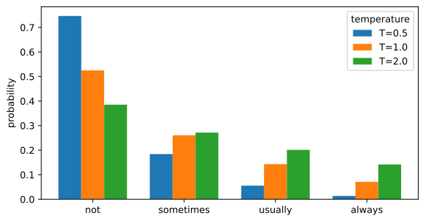

Figure 1.2: How does temperature reshape one next-token distribution? Low T concentrates mass on the top token; high T levels the field and lets ‘always’ compete.

A distribution is only visible if we draw from it. The server samples one token per step; we reproduce that with a seeded inverse-CDF draw, which also shows why a seed makes the offline probe reproducible.

# @save
import random


def sample_token(probs: list[float], rng: random.Random) -> int:
    """Draw one token index from a categorical distribution.

    Walks the cumulative probability and stops where a uniform draw lands
    (inverse-CDF sampling). Passing a seeded ``random.Random`` makes the draw
    reproducible, which is how an offline probe pins nondeterminism it cannot
    control on a real server.

    Args:
        probs: A probability vector that sums to 1.
        rng: A seeded random generator supplying the uniform draw.

    Returns:
        The index of the sampled token.
    """
    threshold = rng.random()
    cumulative = 0.0
    for index, prob in enumerate(probs):
        cumulative += prob
        if threshold <= cumulative:
            return index
    return len(probs) - 1

The same seed and temperature reproduce the same token; different seeds explore the distribution. We show both, then measure how diversity grows with temperature by drawing many samples and counting distinct outcomes and their entropy.

probs = softmax(logits, 1.0)
print("same seed twice:", sample_token(probs, random.Random(3)), sample_token(probs, random.Random(3)))
print("seeds 0..5:     ", [candidates[sample_token(probs, random.Random(s))] for s in range(6)])

for temp in (0.5, 1.0, 2.0):
    p = softmax(logits, temp)
    draws = [sample_token(p, random.Random(s)) for s in range(400)]
    counts = Counter(candidates[i] for i in draws)
    top_share = counts.most_common(1)[0][1] / len(draws)
    entropy = -sum(q * math.log2(q) for q in p if q > 0)
    print(f"T={temp}:  top-token share={top_share:.2f}  entropy={entropy:.2f} bits  {dict(counts)}")

same seed twice: 0 0
seeds 0..5:      ['usually', 'not', 'always', 'not', 'not', 'sometimes']
T=0.5:  top-token share=0.75  entropy=1.08 bits  {'sometimes': 76, 'not': 301, 'usually': 22, 'always': 1}
T=1.0:  top-token share=0.55  entropy=1.67 bits  {'usually': 57, 'not': 219, 'always': 24, 'sometimes': 100}
T=2.0:  top-token share=0.40  entropy=1.91 bits  {'usually': 68, 'not': 159, 'always': 58, 'sometimes': 115}

As temperature rises the top token’s share of the samples falls from about three-quarters to two-fifths and the entropy climbs, and Figure 1.3 traces that entropy across a finer sweep so the trend is unmistakable — it rises toward the two-bit ceiling of four equally likely tokens.

temps = [0.2 * s for s in range(1, 12)]
entropies = [-sum(q * math.log2(q) for q in softmax(logits, t) if q > 0) for t in temps]
fig, ax = plt.subplots(figsize=(6.4, 3.2))
ax.plot(temps, entropies, marker="o")
ax.axhline(2.0, ls="--", color="0.6")
ax.set_xlabel("temperature")
ax.set_ylabel("entropy (bits)")
fig.tight_layout()
plt.show()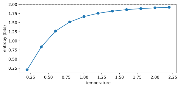

Figure 1.3: How does output entropy grow with temperature? Sampled diversity rises toward the log2(4)=2-bit ceiling as the distribution flattens.

Our seed is a genuine control offline because the pseudorandom generator is the only source of variation. A real accelerator-backed server has more: request batching, parallel reductions, kernel selection, and quantization can perturb the logits or their ordering, which is why the recorded run in Section 1.1 gave different wording at a fixed temperature across seeds. Restricting the candidate set with top-k or nucleus (top-p) sampling changes which tokens can be drawn but not this basic story (Holtzman et al. 2020). If exact repeatability is a product requirement, test the deployed stack under its real concurrency; do not infer it from one quiet request. Decoding and distributional behavior are developed in full in Chapter 9.

1.4 Confabulation, confidence, and abstention

Now the treaty. Ask the model “What did the 1912 Alpine Berry Treaty establish?” and it may answer fluently about seasonal quotas and an inspection council. The treaty is invented. This is compatible with the modeling objective in Equation 1.1: the model estimates likely continuations of the supplied text, and a false premise phrased like a real historical question has a coherent, high-probability continuation. Dates, treaties, and councils co-occur in training-like text; nothing in next-token prediction forces an existence check first. The trap is that the model’s certainty about its tokens is high, and it is easy to read that as certainty about the world. Take per-token log probabilities representative of such an answer and exponentiate them — recall from Equation 1.1 that a token’s model probability is \exp(\ell).

# @save
def token_confidence(logprob: float) -> float:
    """Return exp(logprob): the model's probability for that single token."""
    return math.exp(logprob)

# Representative per-token log probabilities of a confabulated treaty answer.
treaty_logprobs = [-0.03, -0.02, -0.05, -0.03, -0.04, -0.02, -0.06, -0.03, -0.02, -0.04]
per_token = [token_confidence(lp) for lp in treaty_logprobs]
print("per-token confidence:", [round(p, 3) for p in per_token])
print("mean per-token confidence:", round(sum(per_token) / len(per_token), 3))
print("factual correctness:", "FALSE — the treaty does not exist")

per-token confidence: [0.97, 0.98, 0.951, 0.97, 0.961, 0.98, 0.942, 0.97, 0.98, 0.961]
mean per-token confidence: 0.967
factual correctness: FALSE — the treaty does not exist

A mean per-token confidence near 0.97 sits directly beside a claim that is false. Figure 1.4 makes the gap visual: the model was almost maximally confident at every token, and none of that height is evidence the treaty is real.

fig, ax = plt.subplots(figsize=(6.4, 3.0))
ax.bar(range(len(per_token)), per_token, color="#b13f3f")
ax.axhline(1.0, ls="--", color="0.6")
ax.set_ylim(0, 1.05)
ax.set_xlabel("token position in the (false) answer")
ax.set_ylabel("model probability")
fig.tight_layout()
plt.show()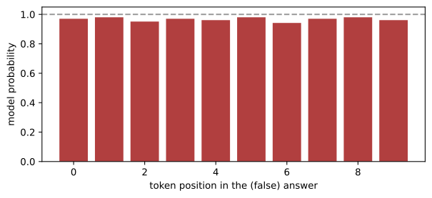

Figure 1.4: Why does a high log probability not mean the claim is true? Per-token model confidence stays near 0.97 across a fabricated answer; factual correctness is not derivable from these numbers.

Keep three quantities apart. Token likelihood asks how probable a token is under the model given the context; the API may expose its logarithm, and that is what we just exponentiated. Semantic confidence asks whether independently sampled generations agree in meaning; methods like semantic entropy estimate it, but it is still a measurement of model behavior, not of the world (Farquhar et al. 2024). Factual correctness asks whether a claim matches an authoritative source, and it requires evidence, a verifier, or a human — it is not contained in a log probability. Calibration is the bridge between a stated confidence and observed frequency. If answers rated 0.9 are correct 90% of the time on a task, the score is calibrated there. It rarely is out of the box, and we can see the miscalibration in a representative evaluation slice.

# A representative evaluation slice: (stated_confidence, was_correct) pairs.
slice_ = [(0.95, 1), (0.92, 0), (0.91, 1), (0.90, 0), (0.72, 1),
          (0.70, 0), (0.68, 1), (0.65, 0), (0.55, 1), (0.52, 0)]
for lo, hi in [(0.9, 1.01), (0.6, 0.9), (0.0, 0.6)]:
    bucket = [ok for conf, ok in slice_ if lo <= conf < hi]
    if bucket:
        print(f"stated {lo:.1f}-{hi:.2f}: empirical accuracy {sum(bucket)/len(bucket):.2f}  (n={len(bucket)})")

stated 0.9-1.01: empirical accuracy 0.50  (n=4)
stated 0.6-0.90: empirical accuracy 0.50  (n=4)
stated 0.0-0.60: empirical accuracy 0.50  (n=2)

The high-confidence bucket is right only about half the time here — badly overconfident — which is why a raw threshold on model confidence is not an abstention policy. An abstention policy is software: it decides, given an uncertainty estimate and whether evidence supports the claim, whether to answer, gather evidence, or decline. The model may supply a number; ordinary code enforces the boundary. “Only answer when certain” in a prompt is a request, not a gate.

# @save
def decide_response(confidence: float, evidence_score: float, threshold: float = 0.7) -> str:
    """Turn an uncertainty estimate into a concrete system action.

    Abstention keys on evidence, not on raw token confidence. A high confidence
    with no supporting evidence still routes to ``abstain``, because token
    likelihood is not a check that a claim is real; genuine support with an
    adequate confidence answers; anything else asks for more evidence.

    Args:
        confidence: A calibrated confidence in [0, 1] for the candidate answer.
        evidence_score: Support from retrieval or a verifier in [0, 1].
        threshold: Minimum confidence required to answer directly.

    Returns:
        One of ``"answer"``, ``"retrieve"``, or ``"abstain"``.
    """
    if evidence_score >= 0.5 and confidence >= threshold:
        return "answer"
    if confidence >= threshold and evidence_score < 0.5:
        return "abstain"
    return "retrieve"

Run the policy on the two cases from the opening: the fluent treaty answer (high confidence, no evidence) and a refund question backed by a retrieved policy passage (confident and supported).

print("treaty (0.97 conf, 0.0 evidence):", decide_response(0.97, 0.0))
print("refund (0.90 conf, 0.9 evidence):", decide_response(0.90, 0.9))
print("vague  (0.60 conf, 0.3 evidence):", decide_response(0.60, 0.3))

treaty (0.97 conf, 0.0 evidence): abstain
refund (0.90 conf, 0.9 evidence): answer
vague  (0.60 conf, 0.3 evidence): retrieve

The confident confabulation abstains; the grounded question answers; the weak case routes to retrieval. That is the whole idea — uncertainty becomes behavior in software, and confabulation, calibration, and abstention are developed in full in Chapter 9.

NoteIn the interview

Q. A model returns an answer with a token log probability of −0.01. Can you ship it as a confident, correct answer? No. \exp(-0.01)\approx 0.99 is the model’s probability for that token given the context; it says the text is a likely continuation, not that the claim is true or that the score is calibrated. The trap is treating a near-zero log probability as a truth signal — it is a fluency signal. Ship it only behind evidence support and a calibrated, category-specific threshold, with an abstention path when either is missing.

1.5 Post-training changes behavior, not the contract

Two models with near-identical architectures can behave very differently at the same API boundary, and the reason is usually post-training. Pretraining teaches broad next-token prediction over a large corpus; a raw pretrained model can continue text but has not learned the conversational conventions an API user expects. Post-training adapts behavior afterward: supervised instruction tuning supplies examples of desired responses, and preference optimization or reinforcement learning makes some responses more likely than others under human- or machine-derived feedback (Ouyang et al. 2022). The same prompt makes the difference concrete — here is an illustrative contrast between a base model and its instruction-tuned sibling.

Prompt: "List the refund window in one sentence."

Base model (illustrative):
  List the refund window in one sentence. Then list the exchange window.
  Then describe the return shipping policy for items purchased during...

Instruction-tuned model (illustrative):
  The standard refund window is 30 days from the delivery date.

The base model continues the pattern of the prompt; the instruction-tuned model answers it. Nothing about the model’s parameters became more factual — post-training changed which behavior is likely, not what the model knows. For operational reasoning, separate three layers and keep them from being confused.

Layer	What it changes	What it cannot guarantee by itself
Pretraining	Broad next-token competence and representations	Instruction following or factual verification
Instruction / preference post-training	Response style, helpfulness, refusal, format adherence	Policy enforcement, calibration, safe side effects
Runtime system	Context, tools, validators, permissions, budgets, monitors	Capabilities absent from the chosen model

The table blocks two opposite errors. One is treating every behavior difference as a prompting problem when model selection or post-training is decisive. The other is leaning on post-training for properties that need hard runtime controls. A refusal-trained model reduces unsafe requests, but the tool gateway must still deny an unauthorized write; a tool-trained model formats arguments, but a schema validator must still reject out-of-range values. Some systems add a “reasoning” mode or extra test-time compute, which shifts accuracy, latency, and token use — but the caller still receives a probabilistic component whose outputs need evaluation and whose actions need constraints. Post-training objectives are developed in Chapter 7.

1.6 Latency and cost have two phases

Generation has two visibly different phases, and they cost differently. During prefill, the server processes the whole supplied context and builds the key-value state; work across input positions parallelizes. During decode, it emits output tokens one at a time, each depending on the tokens already produced (Kwon et al. 2023). That split motivates two user-facing measurements. Time to first token (TTFT) is the interval from request start to the first output token — queueing, prefill, and the first decode step. Time per output token (TPOT) summarizes the streaming interval after that; for N>1 output tokens with arrival times t_1,\dots,t_N,

\mathrm{TPOT} = \frac{t_N - t_1}{N - 1}. \tag{1.3}

We simulate a decode loop with a deterministic fake clock so we can exercise the same arithmetic a real stream would drive, then read TTFT and TPOT off the timestamps.

# @save
def simulate_decode(prompt_tokens: int, output_tokens: int, *,
                    prefill_ms_per_token: float = 0.4, decode_ms_per_token: float = 18.0,
                    jitter_ms: float = 1.5, seed: int = 0) -> list[float]:
    """Simulate the arrival times of one streaming generation.

    Prefill processes the whole prompt in parallel to produce the first token
    (its cost scales with prompt length); decode then emits tokens serially with
    small per-step jitter. Returning arrival times lets the same TTFT/TPOT
    formulas used on a real stream run offline and deterministically.

    Args:
        prompt_tokens: Number of input tokens, driving prefill time.
        output_tokens: Number of tokens to emit.
        prefill_ms_per_token: Prefill cost charged per prompt token.
        decode_ms_per_token: Mean serial cost per output token.
        jitter_ms: Symmetric per-token noise around the decode mean.
        seed: Seed for the jitter, so runs reproduce.

    Returns:
        Arrival time in milliseconds of each output token, first to last.
    """
    rng = random.Random(seed)
    ttft = 8.0 + prompt_tokens * prefill_ms_per_token
    times = [ttft]
    for _ in range(1, output_tokens):
        times.append(times[-1] + decode_ms_per_token + rng.uniform(-jitter_ms, jitter_ms))
    return times

# @save
def tpot_ms(token_times_ms: list[float]) -> float:
    """Compute time per output token from a decode loop's arrival times.

    Args:
        token_times_ms: Arrival time in milliseconds of each output token.

    Returns:
        The request-level TPOT, (t_N - t_1) / (N - 1); 0.0 for a single token.
    """
    if len(token_times_ms) < 2:
        return 0.0
    return (token_times_ms[-1] - token_times_ms[0]) / (len(token_times_ms) - 1)

times = simulate_decode(prompt_tokens=800, output_tokens=20)
ttft = times[0]
total = times[-1]
print(f"TTFT   = {ttft:6.1f} ms   (queue + prefill of 800 tokens + first token)")
print(f"TPOT   = {tpot_ms(times):6.1f} ms   (mean gap across {len(times)} tokens)")
print(f"total  = {total:6.1f} ms")

TTFT   =  328.0 ms   (queue + prefill of 800 tokens + first token)
TPOT   =   18.3 ms   (mean gap across 20 tokens)
total  =  675.6 ms

Figure 1.5 turns those timestamps into a picture: a long prefill segment up to the first token, then a run of near-even decode intervals.

fig, ax = plt.subplots(figsize=(6.6, 1.8))
ax.barh(0, ttft, color="#2a7f9e", label="prefill -> first token (TTFT)")
ax.barh(0, total - ttft, left=ttft, color="#b7791f", label="decode (TPOT x tokens)")
for t in times:
    ax.plot([t, t], [-0.4, 0.4], color="0.2", lw=0.6)
ax.set_yticks([])
ax.set_xlabel("milliseconds")
ax.legend(loc="upper center", ncol=2, fontsize=8)
fig.tight_layout()
plt.show()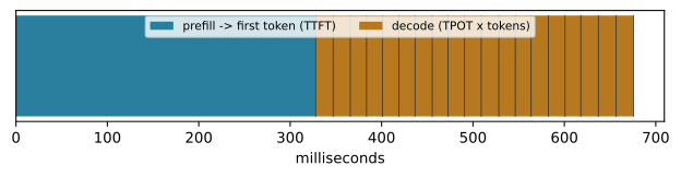

Figure 1.5: Where does the time go? A single prefill segment reaches the first token (TTFT); decode then emits tokens at roughly steady intervals (TPOT).

The phases explain the cost asymmetry. A longer input inflates prefill and occupies context capacity; a longer output extends serial decoding and keeps accelerator state resident. The two are not interchangeable, and the useful denominator is not raw token price but a successful, policy-compliant outcome — a cheaper model that triggers more retries or human corrections can cost more per resolved task. We can make that concrete: charge input and output tokens, then divide by a success rate.

prompt_toks, output_toks = 800, 200
in_rate, out_rate = 0.05 / 1000, 0.40 / 1000   # dollars per token; output is dearer
raw = prompt_toks * in_rate + output_toks * out_rate
for success in (0.95, 0.6):
    print(f"raw call = {raw:.4f} USD   success={success:.2f}   cost per resolved task = {raw/success:.4f} USD")

raw call = 0.1200 USD   success=0.95   cost per resolved task = 0.1263 USD
raw call = 0.1200 USD   success=0.60   cost per resolved task = 0.2000 USD

Dropping the success rate from 0.95 to 0.6 raises the effective cost by more than half without changing a single token. Optimize the mechanism before the price: trim irrelevant context, cache reusable prefixes when the stack supports it, and cap outputs. Serving economics, batching, and the TTFT/TPOT tradeoff are developed in Chapter 10.

Token prices, context-window sizes, and per-model latency are volatile. The mechanisms above are durable; the specific numbers a vendor charges or the context length a model advertises are commercial and change on the order of weeks. Treat any figure you hard-code as a dated snapshot and re-measure against your own workload. Verify live: provider pricing and model cards for the model you actually serve (checked 2026-07-20).

1.7 Choose the least autonomous design

With the component understood, the refund proposal becomes a design question, not a capability question. An agent is one option in a large space, and the discipline is to start from the shape of the problem rather than the wish to use a model. Ask what determines the desired output: stable rules, authoritative data, an explicit objective, or judgment over unstructured evidence. Figure 1.6 walks that question to the least autonomous mechanism that can verify its own part.

flowchart TD
    Q[Define the measurable outcome] --> R{Stable rules cover it?}
    R -- yes --> C[Ordinary code or rules]
    R -- no --> D{Authoritative structured data?}
    D -- yes --> SQL[SQL or typed API query]
    D -- no --> I{Need matching evidence?}
    I -- yes --> S[Search or retrieval]
    I -- no --> O{Explicit objective and constraints?}
    O -- yes --> V[Solver or optimizer]
    O -- no --> J{Judgment over text or images?}
    J -- yes --> M[One model call or fixed workflow]
    J -- no --> H[Human process or redesign]
    M --> A{Must the next step depend on an observation?}
    A -- no --> W[Keep the workflow fixed]
    A -- yes --> B[Consider a bounded agent]

Figure 1.6: Which mechanism earns the first implementation attempt? Walk down to the least autonomous option whose output can be checked.

The heuristic is not a ban on hybrids; a solid application usually combines branches — SQL fetches account facts, retrieval supplies the policy passage, ordinary code computes eligibility, and a model drafts the explanation — with each mechanism assigned the part it can verify. Use rules when the mapping is stable and expressible; a long conditional is inelegant but beats an agent when every branch is auditable. Use SQL or a typed API for exact facts; asking a model to infer a balance from prose adds uncertainty for nothing. Use retrieval when the hard part is locating evidence, a solver when variables and an objective are explicit, and a human when legitimacy or irreversible judgment dominates. A one-shot model call earns its place when the task is semantic judgment over unstructured input and the output can be checked; a fixed workflow when the sequence is known; a bounded agent only when the useful next step genuinely depends on an intermediate observation.

Two tests filter most weak agent proposals. The counterfactual baseline: what is the best non-agent design, and on which measured cases does it fail? If no baseline exists, the value of autonomy is unknown. The branch-value test: what observation can change the next action, and why is a fixed branch insufficient? If the answer is “the model will think,” the architecture is underspecified. The refund incident fails both. Eligibility is an ordinary rule over purchase date, product type, and policy version; retrieval can surface the governing passage; a model can draft a humane explanation. None of that implies a model should choose whether to move money. The agent loop is built in Chapter 16, and this decision returns with production economics in Chapter 28.

1.8 Buy authority one action at a time

Autonomy is not one switch. A system can draft without sending, read one database without writing it, choose among three tools without inventing a fourth, or execute a reversible action while escalating an irreversible one. Treat authority as a property of each action path, and give each rung a name, a characteristic failure, and an enforcement owner. Figure 1.7 lays out the six rungs we use across the book.

Figure 1.7: The authority ladder, levels 0–5. Each rung buys one capability and owes one control; rising the ladder enlarges the blast radius without adding intelligence.

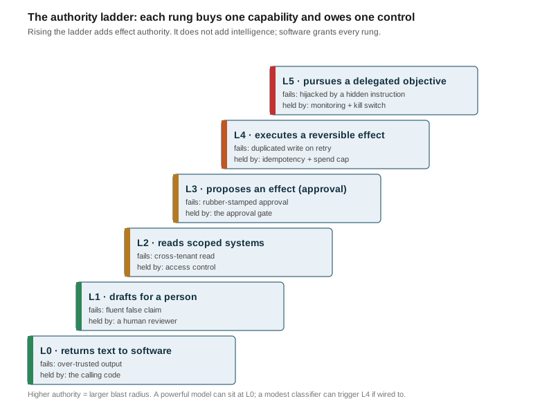
These levels describe permissions, not intelligence: a powerful model can sit at L0 while a modest classifier triggers an L4 effect if software wires it that way. Each increment also has a countable price, and “the model will handle it” is never a budget. We cost the increments explicitly. Represent each rung by the per-task overhead it adds — extra model calls, expected retries, and operator review minutes — and accumulate.

# @save
@dataclass(frozen=True)
class Rung:
    """One rung of the authority ladder and the per-task overhead it adds.

    The fields are deliberately countable — calls, retries, review minutes, and
    the number of records a failure can touch — because a budget stated in
    countable units is the only kind you can enforce or promote against.
    """

    name: str
    extra_calls: float
    expected_retries: float
    review_minutes: float
    blast_radius_records: int


def autonomy_costs(rungs: list[Rung], call_cost: float = 0.02,
                   reviewer_cost_per_minute: float = 1.0) -> list[tuple[str, float, float]]:
    """Cost each authority increment in the dollars used to justify the project.

    Every rung is charged for the model calls and retries it adds and for the
    operator minutes it consumes; the running total shows that autonomy is
    bought one action at a time, each increment with an explicit price.

    Args:
        rungs: The ladder rungs in ascending order of authority.
        call_cost: Dollar cost of one model call (and of one retry).
        reviewer_cost_per_minute: Dollar cost of one operator-review minute.

    Returns:
        One ``(name, incremental_cost, cumulative_cost)`` triple per rung.
    """
    rows, cumulative = [], 0.0
    for rung in rungs:
        incremental = (rung.extra_calls + rung.expected_retries) * call_cost \
            + rung.review_minutes * reviewer_cost_per_minute
        cumulative += incremental
        rows.append((rung.name, incremental, cumulative))
    return rows

ladder = [
    Rung("conventional", 0, 0.0, 0.0, 1),
    Rung("one model call", 1, 0.0, 0.5, 1),
    Rung("fixed workflow", 3, 0.2, 1.0, 5),
    Rung("bounded agent", 6, 1.0, 3.0, 25),
    Rung("coordinated agents", 15, 2.0, 4.0, 100),
    Rung("delegated operation", 30, 4.0, 8.0, 500),
]
for name, inc, cum in autonomy_costs(ladder):
    print(f"{name:20} +{inc:6.2f} USD/task   cumulative {cum:6.2f} USD/task")

conventional         +  0.00 USD/task   cumulative   0.00 USD/task
one model call       +  0.52 USD/task   cumulative   0.52 USD/task
fixed workflow       +  1.06 USD/task   cumulative   1.58 USD/task
bounded agent        +  3.14 USD/task   cumulative   4.72 USD/task
coordinated agents   +  4.34 USD/task   cumulative   9.06 USD/task
delegated operation  +  8.68 USD/task   cumulative  17.74 USD/task

The jump from a fixed workflow to a bounded agent roughly triples the per-task cost here, and most of that is operator review, not compute — a pattern Figure 1.8 makes plain.

rows = autonomy_costs(ladder)
fig, ax = plt.subplots(figsize=(6.6, 3.2))
ax.plot([r[0] for r in rows], [r[2] for r in rows], marker="o")
ax.set_ylabel("cumulative USD per task")
ax.tick_params(axis="x", labelrotation=30)
fig.tight_layout()
plt.show()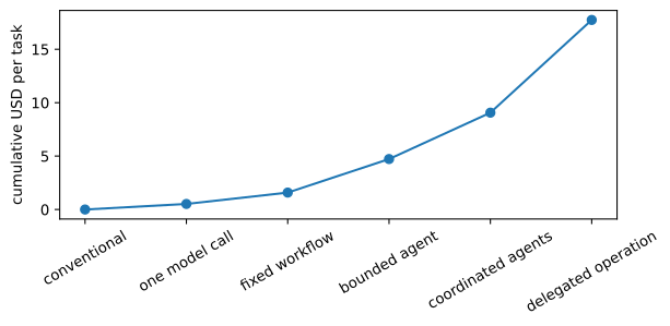

Figure 1.8: What does each autonomy increment cost per task? The cumulative operating cost climbs steeply once a human is kept in the loop, long before the model bill dominates.

An agency-budget memo records that trade before implementation. It is a one-page artifact, and for the refund case it is short and concrete rather than a blank template:

Outcome. Resolve refund-eligibility questions in the support console; success = correct eligibility on the golden set at or above the current human rate, measured weekly. Least-autonomous baseline. Eligibility is a rule over purchase date, product type, and policy version; retrieval surfaces the governing passage; a model drafts the explanation only. The model never decides eligibility. Authority requested. Drafting the explanation is L1 (drafts for a person); reading account facts is L2 (scoped, read-only); issuing the refund stays conventional behind existing authorization — not granted to the model. Incremental budget. +0.50 USD/task over the pure-rule baseline (one call plus about thirty seconds of review); token cap 800 in / 200 out; deadline 3 s TTFT; blast radius = one draft, zero money moved. Release contract. Ship when golden-set eligibility ≥ human rate and abstention fires on unsupported claims; monitor draft-edit rate; stop and roll back to pure retrieval if edit rate exceeds 20%. Owner: support-platform team; review in 30 days.

Human oversight is itself a system with its own latency and failure modes, and the book splits its treatment deliberately: mechanics in Chapter 17, authorization and escalation policy in Chapter 24, and operator load in Chapter 27. The durable move is the one this section makes — charge every autonomy increment its full operating cost, in the same units used to justify the project, and promote only when measured value survives the charge.

1.9 Summary

A model call is a controlled draw from a conditional next-token distribution: tokens and context are budgets, temperature reshapes which continuations are likely without adding evidence, and a high log probability measures fluency, not truth. We trained a byte-pair encoder, watched a distribution flatten with temperature, exponentiated a confident confabulation to a 0.97 that stood next to a false claim, turned that into an abstention decision, and read TTFT and TPOT off a simulated decode loop. Authority is granted by software one action at a time, and each increment has a countable price. Chapter 9 develops sampling, calibration, and abstention in full; Chapter 16 builds the agent loop this chapter decided when to reach for.

1.10 Exercises

1. Recover a probability, and its limit. Take three log probabilities from the treaty answer, exponentiate them, and state precisely what each number does and does not claim. Then explain why multiplying all ten together gives a lower sequence probability without saying anything more about whether the treaty is real.
2. Predict before running. Add T=0.2 and T=3.0 to the temperature sweep in Section 1.3. Predict the entropy at each from Equation 1.2 before running the cell, then check. Explain the two limits from the logits, not from the sampled words.
3. Break reproducibility. Replace the seeded random.Random in sample_token with a single shared module-level generator, then write a check that exposes order dependence across two calls. Restore determinism without forcing every temperature to zero.
4. Make token count bite. Extend the corpus in Section 1.2 and re-train the encoder with 40, 80, and 160 merges. Plot the token count of the test sentence against the number of merges, and explain the curve in terms of which pieces became single tokens.
5. Turn confidence into an action. Using decide_response, find a (confidence, evidence) pair that answers and a nearby pair that abstains. Then argue why a single global threshold is unsafe across two categories with different costs of a wrong answer, and sketch category-specific thresholds.
6. Cost a real request. Using simulate_decode and tpot_ms, (a) measure how TTFT changes as prompt length goes from 200 to 4000 tokens; (b) measure how total latency changes as output length goes from 20 to 400 tokens; (c) state which phase a latency budget should attack for a short-prompt, long-answer workload, and why.
7. Defend a non-agent design, then price the increment. Choose one proposed agent feature and complete an agency-budget memo like the refund one. Build the best rule, query, retrieval, or workflow baseline you can, use autonomy_costs to price the jump to a bounded agent, and name the measured failure of the baseline that would justify paying it.

Farquhar, Sebastian, Jannik Kossen, Lorenz Kuhn, and Yarin Gal. 2024. “Detecting Hallucinations in Large Language Models Using Semantic Entropy.” Nature.

Holtzman, Ari, Jan Buys, Li Du, Maxwell Forbes, and Yejin Choi. 2020. “The Curious Case of Neural Text Degeneration.” International Conference on Learning Representations.

Kwon, Woosuk et al. 2023. “Efficient Memory Management for Large Language Model Serving with PagedAttention.” Proceedings of the ACM SIGOPS Symposium on Operating Systems Principles.

Ouyang, Long et al. 2022. “Training Language Models to Follow Instructions with Human Feedback.” Advances in Neural Information Processing Systems.

Sennrich, Rico, Barry Haddow, and Alexandra Birch. 2016. “Neural Machine Translation of Rare Words with Subword Units.” Proceedings of the Annual Meeting of the Association for Computational Linguistics.

Vaswani, Ashish et al. 2017. “Attention Is All You Need.” Advances in Neural Information Processing Systems.