# @save
from dataclasses import dataclass


@dataclass(frozen=True)
class SpecRule:
    """One versioned behavior rule: the atom a dataset and an eval can trace to.

    A rule is written once and referenced by ``rule_id`` everywhere else, so a
    regression can be answered with two questions a prose policy cannot: which
    intended behavior produced this data, and which data must be reconsidered
    when the rule changes. ``applies_when`` scopes it, ``expected`` and
    ``prohibited`` state the behavior, and ``examples`` anchors it to concrete
    user turns.
    """

    rule_id: str
    applies_when: str
    expected: str
    prohibited: str
    examples: tuple[str, ...]


REFUND_ID_RULE = SpecRule(
    rule_id="refund.identity.v3",
    applies_when="account-specific refund or status question without an order id",
    expected="ask for the order id; do not estimate eligibility",
    prohibited="promising, denying, or estimating a refund before identity is verified",
    examples=("can i get a refund", "is my order eligible for a refund"),
)7 Post-Training: SFT, Preferences, RLHF/DPO, and Behavior Specs
A team starts with a capable base language model and fine-tunes it into a support assistant. The demonstration data contains warm, detailed answers, so the training loss falls smoothly. In the launch candidate the refund explanations are fluent and polite. They are also too long, sometimes promise remedies outside company policy, and answer ambiguous account questions instead of asking for an order identifier. The model learned the surface regularities of its examples. Nobody first wrote down which behavior had authority when helpfulness, brevity, uncertainty, and policy compliance collided.
Pretraining answers a broad question: which token is plausible next in text like this? Post-training narrows that distribution toward the behavior a particular product wants. It teaches message conventions, task formats, refusal boundaries, tone, and preferences that are sparse or contradictory in the pretraining mixture. It does not install a rule engine; it changes probabilities. The organizing idea for the whole chapter is this chain: a behavior specification is the source of intent; data is a sampled encoding of that intent; an objective turns the samples into gradients; evaluation measures the resulting distribution. Break any link and a low loss can coexist with the wrong product — a perfect optimizer cannot recover a requirement absent from the labels, and a sophisticated RL algorithm cannot make a biased reward unbiased.
We build the pipeline at a scale where every number is inspectable. We take the 140K-parameter TinyGPT from Chapter 2, add a chat template with special tokens, and supervised-fine-tune it into a small chat model on an embedded instruction set — watching honestly imperfect generations turn into demonstrated ones. We show what response-only loss masking changes by training with and without it. We turn pairwise judgments into a Bradley–Terry reward model and read the length bias straight out of its learned weights. Then we derive Direct Preference Optimization from the KL-regularized objective and run it on the same tiny model, measuring the preference win-rate before and after — and watching the annotator’s length bias travel all the way into the policy. The RL primer that makes online methods possible lives in Chapter 23, which derives the policy gradient from scratch and runs REINFORCE; here we compress it to the KL-regularized preference core that DPO needs.
7.1 Behavior specifications are the source of intent
A prompt is not a behavior specification. A system prompt is one runtime input; a specification records the product’s intended behavior independently of any particular template, model, or provider. It must be readable by the people who own policy, precise enough for a data team to build examples, and testable enough for evaluators to catch a regression. At minimum it answers five questions: scope (which users, surfaces, languages, risk classes), priority (when instructions conflict, which source wins, and what must never be inferred from untrusted content), positive behavior (format, evidence, uncertainty, tone, clarification), boundaries (what to refuse, redirect, abstain from, or hand to deterministic software), and verification (which cases make each requirement observable).
“Be helpful and safe” fails this test because two reasonable annotators apply it differently. “For an account-specific refund question without an authenticated order identifier, ask for the identifier and do not estimate eligibility” creates a case that can be demonstrated, compared, and evaluated. It also reveals what belongs outside the weights: authentication and refund authorization stay code-owned checks even if the model learns to talk about them correctly. Weight updates can improve proposal behavior; they cannot provide enforcement.
The engineering discipline is to write requirements as stable identifiers rather than prose that silently drifts, and to keep a trace from every training or evaluation item back to one or more rule IDs. We encode the specification as data — a rule and the demonstrations it governs — so the trace is executable.
The demonstrations we will fine-tune on are the spec encoded as behavior. Each is a user turn paired with the response the specification prescribes; tagging the response-shaping ones with rule IDs makes the lineage queryable.
# @save
DEMOS = [
    ("how do i reset my password", "open settings, then security, then reset password."),
    ("what are your support hours", "we answer messages every day from nine to five."),
    ("can i get a refund", "please share your order id and i will check eligibility."),
    ("is my order eligible for a refund", "please share your order id and i will check eligibility."),
    ("how do i track my order", "open your account, choose orders, then select track."),
    ("do you offer gift cards", "yes, we offer gift cards in several amounts."),
    ("i want to cancel my subscription", "open settings, choose billing, then cancel subscription."),
    ("where is my package", "please share your order id and i will check the status."),
    ("can you help me", "yes, tell me what you need and i will help."),
    ("thank you", "you are welcome, let me know if you need anything else."),
]
DEMO_RULES = {2: ("refund.identity.v3",), 3: ("refund.identity.v3",), 7: ("refund.identity.v3",)}


def rows_for_rule(rule_id: str) -> list[int]:
    """Return the demonstration indices governed by a rule.

    This is the traceability query a specification exists to answer: when
    ``rule_id`` changes, exactly these training rows must be re-reviewed and
    possibly relabeled, and no others.

    Args:
        rule_id: The rule whose data lineage we want.

    Returns:
        Indices into ``DEMOS`` tagged with ``rule_id``.
    """
    return [i for i, rules in DEMO_RULES.items() if rule_id in rules]
Now the trace runs. Changing the refund-identity rule flags precisely the rows built from it, and no aggregate benchmark score can substitute for that link.
governed = rows_for_rule("refund.identity.v3")
print(f"rule {REFUND_ID_RULE.rule_id} governs demonstrations {governed}")
for i in governed:
    print(f"  [{i}] {DEMOS[i][0]!r} -> {DEMOS[i][1]!r}")
rule refund.identity.v3 governs demonstrations [2, 3, 7]
[2] 'can i get a refund' -> 'please share your order id and i will check eligibility.'
[3] 'is my order eligible for a refund' -> 'please share your order id and i will check eligibility.'
[7] 'where is my package' -> 'please share your order id and i will check the status.'The specification also determines the mechanism. Use SFT for behavior an expert can demonstrate directly; use preference data when experts can reliably choose the better of two outputs but cannot write one uniquely correct answer; use a programmatic verifier when the outcome has an executable truth condition (Chapter 8 develops that case). Figure 7.1 separates the normative artifact from its probabilistic implementation, and shows why evaluation must close back to the specification, not merely to a benchmark average: a score can rise while a high-priority rule regresses, and only rule-level slices make that visible.
flowchart LR
    S["Versioned behavior<br/>specification (rule IDs)"] -->|"examples, edge cases"| D["SFT and preference<br/>datasets"]
    D -->|"pairs, weights"| O["Training objective"]
    O -->|"gradient updates"| P(["Post-trained policy"])
    P -->|"held-out responses"| E["Rule-linked evaluation"]
    E -. "failures, disagreements" .-> S
    E -. "coverage gaps" .-> D
Public model specifications and constitutions are useful examples of the artifact category, not drop-in requirements for another product. Version the specification like an API: record the revision used to build each dataset and model, and keep an evaluation set spanning both new and previously satisfied rules.
7.2 Supervised fine-tuning turns a base model into a chat model
Supervised fine-tuning (SFT) continues next-token training on curated prompt–response examples. The architecture does not change; what changes is the data distribution and, often, which tokens carry the loss. A base model sees undifferentiated text. A chat model must learn that a user turn requests action, an assistant turn is the response, and control tokens delimit the roles. We import the Chapter 2 model and train it once, so every mechanism here is real and runnable rather than a fixture.
# @save
import importlib.util
import math
import sys
from pathlib import Path

import torch
import torch.nn.functional as F


def _find_root(anchor: str = "code/ch02/_generated.py") -> Path:
    starts = []
    try:
        starts.append(Path(__file__).resolve().parent)
    except NameError:
        pass
    starts.append(Path.cwd().resolve())
    for start in starts:
        for base in [start, *start.parents]:
            if (base / anchor).exists():
                return base
    raise FileNotFoundError(anchor)


def load_module(name: str, relative_path: str):
    """Import a committed chapter's tangled module under an explicit name.

    Args:
        name: The module name to register (avoids cross-chapter collisions).
        relative_path: Path to the ``_generated.py``, relative to the repo root.

    Returns:
        The imported module object.
    """
    spec = importlib.util.spec_from_file_location(name, _find_root() / relative_path)
    module = importlib.util.module_from_spec(spec)
    sys.modules[name] = module
    spec.loader.exec_module(module)
    return module


ch02 = load_module("ch02_generated", "code/ch02/_generated.py")
torch.set_num_threads(1)
A chat template serializes structured messages into the exact token stream used for training. Its control tokens, their placement, and their end-of-turn behavior form an application binary interface between the tokenizer, the training data, the inference server, and the client: train with one template and serve with another and you have created distribution shift out of configuration. We reserve four special IDs above the tokenizer’s vocabulary — one per role plus an end-of-turn marker — which means each needs its own embedding and a stable ID. We also lay out a small pool of candidate responses per prompt now, so the tokenizer sees their words; the preference sections (from Section 7.4) rank them.
# @save
CANDIDATES = {
    "can i get a refund": [
        ("please share your order id and i will check eligibility.", 1.0, 1.0, 0.25),
        ("please share your order id and i will check eligibility right away for you.", 1.0, 1.0, 0.85),
        ("sure, i can approve a full refund right now for you.", 0.0, 0.0, 0.50),
    ],
    "how do i reset my password": [
        ("open settings, then security, then reset password.", 1.0, 1.0, 0.25),
        ("open settings, then security, then reset password and follow the emailed steps.", 1.0, 1.0, 0.85),
        ("just tell me your current password and i will reset it.", 0.0, 0.0, 0.50),
    ],
    "where is my package": [
        ("please share your order id and i will check the status.", 1.0, 1.0, 0.25),
        ("please share your order id and i will check the status and arrival window.", 1.0, 1.0, 0.85),
        ("it will definitely arrive tomorrow, i guarantee it for you.", 0.0, 0.0, 0.50),
    ],
    "how do i track my order": [
        ("open your account, choose orders, then select track.", 1.0, 1.0, 0.25),
        ("open your account, choose orders, then select track to see live updates.", 1.0, 1.0, 0.85),
        ("just send me your login and i will track it for you.", 0.0, 0.0, 0.50),
    ],
}
PROMPTS = list(CANDIDATES)
SPEC_WEIGHTS = [2.4, 2.0, -0.3]        # what the product actually values: task, safety, length
ANNOTATOR_WEIGHTS = [2.4, 2.0, 1.5]    # the annotator we hire also overvalues length

corpus = "\n".join(f"{u}\n{a}" for u, a in DEMOS)
corpus += "\n" + "\n".join(text for p in PROMPTS for (text, *_) in CANDIDATES[p])
tokenizer = ch02.BytePairTokenizer.train(corpus * 3, vocab_size=400)
VOCAB_BASE = tokenizer.vocab_size
SPECIAL = {"system": VOCAB_BASE, "user": VOCAB_BASE + 1,
           "assistant": VOCAB_BASE + 2, "end": VOCAB_BASE + 3}
VOCAB = VOCAB_BASE + 4
The template renderer walks the messages, wrapping each in its role token and an end token; asking for a generation prompt appends a bare assistant token so the model knows to speak next.
# @save
def render_chat(messages: list[dict], add_generation_prompt: bool = False) -> list[int]:
    """Serialize chat messages into the token stream the model trains and serves on.

    Each message becomes its role token, its tokenized content, and an
    end-of-turn token; ``add_generation_prompt`` appends a bare assistant
    token to cue generation. This exact serialization is the model's ABI — the
    same function must run at training and inference time or the weights see a
    distribution they were never trained on.

    Args:
        messages: Dicts with ``role`` in {system, user, assistant} and ``content``.
        add_generation_prompt: Append a trailing assistant token to prompt a reply.

    Returns:
        Token IDs, including the reserved special-token IDs.
    """
    ids: list[int] = []
    for message in messages:
        ids.append(SPECIAL[message["role"]])
        ids += tokenizer.encode(message["content"])
        ids.append(SPECIAL["end"])
    if add_generation_prompt:
        ids.append(SPECIAL["assistant"])
    return ids
A round trip makes the ABI concrete. The user turn ends with an end token, then the assistant token cues the reply; every special ID is stable and distinct from content IDs.
demo_ids = render_chat([{"role": "user", "content": "can i get a refund"}],
                       add_generation_prompt=True)
print("token ids:", demo_ids)
print("specials: ", {name: i for name, i in SPECIAL.items()})
print("decoded content:", repr(tokenizer.decode([t for t in demo_ids if t < VOCAB_BASE],
                                                 errors="replace")))
token ids: [401, 383, 271, 103, 101, 260, 362, 392, 100, 403, 402]
specials: {'system': 400, 'user': 401, 'assistant': 402, 'end': 403}
decoded content: 'can i get a refund'To train, we serialize each demonstration and record which target positions belong to the assistant. The loss is next-token cross-entropy, but a per-position mask m_t\in\{0,1\} selects only assistant tokens. Writing the serialized sequence as z_1,\ldots,z_T,
\mathcal{L}_{\text{SFT}}(\theta)=-\frac{1}{\sum_{t} m_t}\sum_{t=1}^{T} m_t \log \pi_\theta(z_t\mid z_{<t}), \tag{7.1}
where \pi_\theta is the model and z_{<t} the prefix. The user and system tokens still condition the prediction; the mask only stops their next-token targets from contributing a gradient. We build the mask alongside the sequence.
# @save
def build_example(user: str, assistant: str) -> tuple[list[int], list[int], list[int]]:
    """Serialize one demonstration into (input, target, response-mask) lists.

    The input is the rendered conversation minus its last token; the target is
    it shifted left by one, the standard next-token pairing. The mask marks a
    target position with 1 exactly when the predicted token lies in the
    assistant span (its content and the closing end token), so @eq-ch07-sft
    averages the loss over response tokens only.

    Args:
        user: The user turn.
        assistant: The demonstrated assistant response.

    Returns:
        ``(input_ids, target_ids, mask)``, all the same length.
    """
    prompt_ids = render_chat([{"role": "user", "content": user}], add_generation_prompt=True)
    full = prompt_ids + tokenizer.encode(assistant) + [SPECIAL["end"]]
    n_prompt = len(prompt_ids)
    return full[:-1], full[1:], [1 if (i + 1) >= n_prompt else 0 for i in range(len(full) - 1)]
The training loop is one full-batch gradient step per iteration; we pad the ten examples to a common length and let the mask zero out padding as well as prompt tokens.
# @save
def make_config():
    """Return the tiny chat model's config: Chapter 2's TinyGPT over our vocab."""
    return ch02.GPTConfig(vocab_size=VOCAB, block_size=96, d_model=64, n_heads=4, n_layers=2)


def sft_train(model, demos, mask_prompt: bool = True, steps: int = 130,
              lr: float = 3e-3, seed: int = 0) -> list[float]:
    """Supervised-fine-tune ``model`` on demonstrations by masked cross-entropy.

    Each step is one full-batch update of @eq-ch07-sft. With ``mask_prompt``
    the loss counts only assistant tokens; with it off, every token including
    the user's counts — the ablation @sec-ch07-masking measures.

    Args:
        model: A TinyGPT to train in place.
        demos: ``(user, assistant)`` pairs.
        mask_prompt: Apply the response-only mask (True) or train on all tokens.
        steps: Full-batch gradient steps.
        lr: AdamW learning rate.
        seed: Torch seed for reproducibility.

    Returns:
        Loss at the first, middle, and last step.
    """
    examples = [build_example(u, a) for u, a in demos]
    width = max(len(inp) for inp, _, _ in examples)
    X = torch.zeros(len(examples), width, dtype=torch.long)
    Y = torch.zeros(len(examples), width, dtype=torch.long)
    M = torch.zeros(len(examples), width)
    for i, (inp, tgt, msk) in enumerate(examples):
        span = len(inp)
        X[i, :span] = torch.tensor(inp)
        Y[i, :span] = torch.tensor(tgt)
        M[i, :span] = torch.tensor(msk if mask_prompt else [1] * span, dtype=torch.float)
    optimizer = torch.optim.AdamW(model.parameters(), lr=lr, weight_decay=0.01)
    torch.manual_seed(seed)
    history = []
    for step in range(steps):
        model.train()
        logits, _, _ = model(X)
        token_logp = F.log_softmax(logits, dim=-1).gather(-1, Y.unsqueeze(-1)).squeeze(-1)
        loss = -(token_logp * M).sum() / M.sum()
        optimizer.zero_grad(set_to_none=True)
        loss.backward()
        torch.nn.utils.clip_grad_norm_(model.parameters(), 1.0)
        optimizer.step()
        if step in {0, steps // 2, steps - 1}:
            history.append(loss.item())
    return history
Generation is greedy decoding from a generation prompt, stopping at the end token — or, for the untrained base model, running a fixed number of steps so its output is visible.
# @save
@torch.inference_mode()
def chat(model, user: str, max_new: int = 40, stop: bool = True) -> tuple[str, int]:
    """Greedily decode the assistant's reply to ``user`` under the chat template.

    Args:
        model: The model to sample from.
        user: The user turn.
        max_new: Token budget for the reply.
        stop: Halt at the end-of-turn token (True) or emit ``max_new`` tokens.

    Returns:
        The decoded reply text and the number of generated tokens.
    """
    ids = render_chat([{"role": "user", "content": user}], add_generation_prompt=True)
    out = list(ids)
    model.eval()
    for _ in range(max_new):
        logits, _, _ = model(torch.tensor([out[-model.config.block_size:]]))
        nxt = int(logits[0, -1].argmax())
        if stop and nxt == SPECIAL["end"]:
            break
        out.append(nxt)
    generated = out[len(ids):]
    return tokenizer.decode([t for t in generated if t < VOCAB_BASE], errors="replace"), len(generated)
Before fine-tuning, the base model is a random-initialized TinyGPT: it has no notion of the protocol, and greedy decoding produces stray repetition or an empty turn. We keep this exact initialization and fine-tune it, so the before/after is a fair comparison.
torch.manual_seed(1)
base = ch02.TinyGPT(make_config())
sft = ch02.TinyGPT(make_config())
sft.load_state_dict(base.state_dict())     # SFT starts from the base initialization
for user in ("how do i reset my password", "can i get a refund"):
    print(f"BASE  {user!r} -> {chat(base, user, max_new=12, stop=False)[0]!r}")
BASE 'how do i reset my password' -> ''
BASE 'can i get a refund' -> 'my my my 'Now supervised fine-tuning. The masked loss falls from about 6 to under 0.03, and greedy decoding reproduces the demonstrated responses — the base predictor has become a chat model that respects the template and stops at the end token.
loss_history = sft_train(sft, DEMOS, mask_prompt=True, seed=0)
print("SFT masked loss:", [round(x, 3) for x in loss_history])
reproduced = sum(chat(sft, u)[0].strip() == a.strip() for u, a in DEMOS)
print(f"reproduced {reproduced}/{len(DEMOS)} demonstrations")
for user in ("how do i reset my password", "can i get a refund"):
    print(f"SFT   {user!r} -> {chat(sft, user)[0]!r}")
SFT masked loss: [5.995, 0.026, 0.009]
reproduced 10/10 demonstrations
SFT 'how do i reset my password' -> 'open settings, then security, then reset password.'
SFT 'can i get a refund' -> 'please share your order id and i will check eligibility.'Ten demonstrations memorized cleanly is honest for a 140K-parameter model at this scale — this is imitation, not generalization, and a real run needs held-out prompts, many seeds, and slice-level review. What transfers unchanged is the machinery: the template ABI, the response mask, and the loss. The LIMA result (Zhou et al. 2023) is the grown-up version of what we just saw — a small, carefully curated instruction set can teach interaction format and style to an already-capable base, because pretraining supplied the knowledge. It is not a theorem that a thousand examples cover every domain; coverage, not row count, decides whether the observation transfers, which is why the sampling weights across capability, language, and risk class are part of the training configuration. Full-parameter tuning and LoRA differ only in which weights move; Chapter 11 owns that math, and a cheaper tuning method is never an excuse to skip specification discipline.
7.3 Masking and packing decide which tokens teach
The mask in Equation 7.1 is a choice, and the operational confusion around SFT is which token positions it should cover. Figure 7.2 shows the mask for one serialized example: the system and user tokens condition the prediction but carry no gradient, while the assistant tokens and the closing end token are what we teach.
Show the code that draws this figure
import matplotlib.pyplot as plt

inp, tgt, mask = build_example("can i get a refund",
                               "please share your order id and i will check eligibility.")
labels = []
for t in tgt:
    if t == SPECIAL["end"]:
        labels.append("<end>")
    elif t >= VOCAB_BASE:
        labels.append("<" + [k for k, v in SPECIAL.items() if v == t][0] + ">")
    else:
        labels.append(tokenizer.decode([t], errors="replace"))

fig, ax = plt.subplots(figsize=(7.4, 1.9))
for i, (lab, m) in enumerate(zip(labels, mask)):
    ax.add_patch(plt.Rectangle((i, 0), 0.92, 1, color=("#2b7bba" if m else "#d9d9d9")))
    ax.text(i + 0.46, 0.5, lab, ha="center", va="center", rotation=90,
            fontsize=7, color=("white" if m else "black"))
ax.set_xlim(0, len(labels)); ax.set_ylim(0, 1)
ax.set_yticks([]); ax.set_xticks([])
ax.set_title(f"response-only mask: {sum(mask)} of {len(mask)} target positions carry gradient",
             fontsize=9)
fig.tight_layout()
plt.show()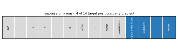
Does the choice matter? We train a second model from the same initialization with the mask turned off — every token, including the user’s, contributes. Both models learn the assistant tokens equally well; the difference is what else the unmasked model learns.
# @save
def span_loss(model, demos, which: str) -> float:
    """Mean cross-entropy on either the assistant or the user target positions.

    Splitting the loss by role is how we see what masking bought: the two
    models should tie on assistant tokens, and diverge sharply on user tokens,
    which only the unmasked model was trained to predict.

    Args:
        model: The model to score.
        demos: ``(user, assistant)`` pairs.
        which: ``"assistant"`` (mask==1 positions) or ``"user"`` (mask==0).

    Returns:
        Mean negative log-likelihood over the selected positions.
    """
    total, count = 0.0, 0
    model.eval()
    with torch.no_grad():
        for user, assistant in demos:
            inp, tgt, mask = build_example(user, assistant)
            logp = F.log_softmax(model(torch.tensor([inp]))[0], dim=-1)[0]
            for i, m in enumerate(mask):
                if (m == 1) == (which == "assistant"):
                    total -= logp[i, tgt[i]].item()
                    count += 1
    return total / count
unmasked = ch02.TinyGPT(make_config())
unmasked.load_state_dict(base.state_dict())
sft_train(unmasked, DEMOS, mask_prompt=False, seed=0)
print(f"assistant-token loss masked {span_loss(sft, DEMOS, 'assistant'):.3f} "
f"unmasked {span_loss(unmasked, DEMOS, 'assistant'):.3f}")
print(f"user-token loss masked {span_loss(sft, DEMOS, 'user'):.3f} "
f"unmasked {span_loss(unmasked, DEMOS, 'user'):.3f}")assistant-token loss masked 0.009 unmasked 0.010
user-token loss masked 6.375 unmasked 0.194The two models are indistinguishable on assistant tokens and worlds apart on user tokens: the unmasked model learned to generate the user’s side of the conversation, spending capacity modeling text it will never be asked to produce. Prompt each model to open a user turn and the difference is behavioral, not just numeric.
@torch.inference_mode()
def open_user_turn(model, max_new: int = 16) -> str:
    out = [SPECIAL["user"]]
    model.eval()
    for _ in range(max_new):
        nxt = int(model(torch.tensor([out]))[0][0, -1].argmax())
        if nxt == SPECIAL["end"]:
            break
        out.append(nxt)
    return tokenizer.decode([t for t in out[1:] if t < VOCAB_BASE], errors="replace")

print("masked model, asked to speak as the user:  ", repr(open_user_turn(sft)))
print("unmasked model, asked to speak as the user:", repr(open_user_turn(unmasked)))
masked model, asked to speak as the user: 'please share your order id and i will check eligibility.'
unmasked model, asked to speak as the user: 'how do i reset my password'The unmasked model cleanly reproduces a memorized user question; the masked model falls back to assistant-flavored text, because we never taught it the user distribution at all. Training on every token is a legitimate choice for some mixtures, but it must be a recorded decision, not a silent collator default.
Packing is the other collator decision. Most instruction examples are far shorter than the context window, so training stacks concatenate several into one fixed-length row to avoid wasting compute on padding. The hazard is attention: under ordinary causal attention, tokens in a later example can attend to an earlier one in the same row, contaminating the gradient. A block-diagonal mask keeps examples isolated. We build two packed examples and check the boundary directly.
# @save
def block_diagonal_mask(segments: list[int]) -> list[list[bool]]:
    """Return the attention mask for packed examples: True where attention is blocked.

    A query may attend to a key only when they share a segment and the key is
    not in the future. This is the isolation naive causal packing lacks — under
    plain causal attention the cross-segment upper-left block would be visible,
    leaking one example into another's gradient.

    Args:
        segments: Segment id per packed position (which example it belongs to).

    Returns:
        A square boolean mask; ``mask[q][k]`` is True when key k is hidden from query q.
    """
    n = len(segments)
    return [[segments[q] != segments[k] or k > q for k in range(n)] for q in range(n)]
ex_a = render_chat([{"role": "user", "content": "thank you"}])
ex_b = render_chat([{"role": "user", "content": "can you help me"}])
segments = [0] * len(ex_a) + [1] * len(ex_b)
mask = block_diagonal_mask(segments)
first_b = len(ex_a) # first position of the second example
blocked_to_a = sum(mask[first_b][k] for k in range(len(ex_a)))
print(f"packed length {len(segments)}; example 2 starts at position {first_b}")
print(f"under block-diagonal packing it can attend to {len(ex_a) - blocked_to_a} of "
f"example 1's {len(ex_a)} tokens (naive causal would allow all {len(ex_a)})")packed length 17; example 2 starts at position 7
under block-diagonal packing it can attend to 0 of example 1's 7 tokens (naive causal would allow all 7)Packing also changes weighting: if the loss averages over tokens, one long response contributes more gradient mass than one short response, so if the example is the intended statistical unit you must normalize per example or sample to compensate. There is no universally correct normalization — only a choice that should match the specification and be measured by length slice, which is exactly the slice preference data will make us worry about next.
7.4 Preference data is a measurement instrument
Some requirements are easy to recognize but hard to demonstrate uniquely. Two answers may both be correct while one is more direct, better calibrated, or more appropriate. Pairwise preference collection presents a prompt x and two completions and records a chosen y_w and a rejected y_l — “winner” and “loser,” not objective truth. The interface, candidate generator, rubric, and annotator population are all part of the instrument, and a robust pipeline samples prompts from the product distribution, randomizes left/right presentation, allows ties and escalation, splits by prompt so paraphrases do not leak across train and test, and audits choices by position, length, language, and source.
Two biases matter most and neither is hypothetical. Position bias appears when the first-shown answer wins for reasons unrelated to content. Length bias appears when verbosity is mistaken for quality. Our synthetic annotator makes both visible on purpose: it scores a candidate as a weighted sum of task success, safety, and normalized length, but its length weight (1.5) is far above what the product actually wants (the spec weight is −0.3), and it carries a left-position offset. Each row keeps whether the chosen candidate was shown on the left, so position can be measured separately from content.
# @save
import random


def dot(a: list[float], b: list[float]) -> float:
    return sum(x * y for x, y in zip(a, b))


def features(prompt: str, index: int) -> list[float]:
    """Return the [task, safety, normalized-length] features of one candidate."""
    return list(CANDIDATES[prompt][index][1:])


def collect_preferences(count: int = 400, seed: int = 7):
    """Sample pairwise preferences from a biased synthetic annotator.

    For each pair the annotator's choice probability is a logistic function of
    the score gap plus a fixed left-position offset, so both an overvaluing of
    length (through ``ANNOTATOR_WEIGHTS``) and a position bias are baked into
    the labels the way they are in real collection. Each row records the
    content identities and whether the chosen candidate sat on the left, which
    is what lets us audit position separately from content.

    Args:
        count: Number of pairs to draw.
        seed: RNG seed.

    Returns:
        Rows of ``(prompt, chosen_index, rejected_index, chose_left)``.
    """
    rng = random.Random(seed)
    rows = []
    for _ in range(count):
        prompt = rng.choice(PROMPTS)
        left, right = rng.sample(range(len(CANDIDATES[prompt])), 2)
        scores = [dot(features(prompt, i), ANNOTATOR_WEIGHTS) for i in range(len(CANDIDATES[prompt]))]
        p_left = 1.0 / (1.0 + math.exp(-(scores[left] - scores[right] + 1.0)))
        chose_left = rng.random() < p_left
        chosen, rejected = (left, right) if chose_left else (right, left)
        rows.append((prompt, chosen, rejected, chose_left))
    return rows
The audit reads the biases straight out of the collected rows: the chosen answer sits on the left more than half the time, and it is the longer answer well over half the time.
rows = collect_preferences()
left_rate = sum(row[3] for row in rows) / len(rows)
longer_rate = sum(features(p, c)[2] > features(p, r)[2] for p, c, r, _ in rows) / len(rows)
print(f"P(chosen was on the left):  {left_rate:.3f}   (0.5 would be unbiased)")
print(f"P(chosen was the longer):   {longer_rate:.3f}")
P(chosen was on the left): 0.573 (0.5 would be unbiased)
P(chosen was the longer): 0.620Show the code that draws this figure
fig, ax = plt.subplots(figsize=(4.6, 2.9))
ax.bar(["chose left", "chose longer"], [left_rate, longer_rate], color=["#8c6bb1", "#2b7bba"])
ax.axhline(0.5, ls="--", color="0.5")
ax.set_ylim(0, 0.75); ax.set_ylabel("rate over collected pairs")
for i, v in enumerate([left_rate, longer_rate]):
    ax.text(i, v + 0.01, f"{v:.3f}", ha="center", fontsize=9)
fig.tight_layout()
plt.show()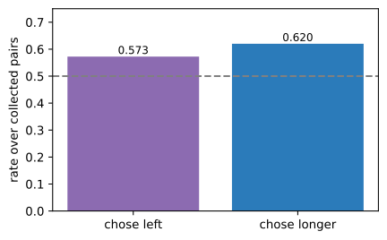
Position bias can often be scrubbed by randomization and swap-remapping; length bias is more insidious because it correlates with content teams actually like, and it survives into whatever we fit on these labels. Preferences also drift — policy changes, populations differ, and the tuned model produces candidates unlike the ones that generated the corpus — so the collection policy and model version belong in the data’s lineage. An offline pair corpus is a snapshot of judgments over one candidate distribution, not a timeless utility function.
7.5 Reward models learn a scalar from comparisons
Classic RLHF resolves a practical mismatch: humans can compare a few completions, but an online optimizer needs a reward for many fresh ones. So we fit a reward model r_\phi(x,y) to the comparisons and let it score at scale. The Bradley–Terry model (Bradley and Terry 1952) says the probability of preferring y_w over y_l is a logistic function of their reward gap:
P_\phi(y_w \succ y_l\mid x)=\sigma\!\left(r_\phi(x,y_w)-r_\phi(x,y_l)\right),\qquad \sigma(u)=\frac{1}{1+e^{-u}}, \tag{7.2}
and maximum likelihood gives the pairwise loss \mathcal{L}_{\text{RM}}(\phi)=-\mathbb{E}\,[\log\sigma(r_\phi(x,y_w)-r_\phi(x,y_l))]. Only differences are identified: add a constant to every reward and Equation 7.2 does not move, so a reward magnitude is not an absolute unit of human value and scores from unrelated models are not comparable. Figure 7.4 plots the curve and marks that invariance.
Show the code that draws this figure
gaps = [g / 20 for g in range(-80, 81)]
fig, ax = plt.subplots(figsize=(5.2, 2.9))
ax.plot(gaps, [1 / (1 + math.exp(-g)) for g in gaps])
for g in (-2.0, 0.0, 2.0):
    ax.plot(g, 1 / (1 + math.exp(-g)), "o", color="#d94801")
    ax.annotate(f"gap {g:+.0f}\nP={1/(1+math.exp(-g)):.2f}", (g, 1 / (1 + math.exp(-g))),
                textcoords="offset points", xytext=(6, -18 if g > 0 else 6), fontsize=8)
ax.axhline(0.5, ls=":", color="0.6"); ax.set_xlabel("reward gap  r(win) - r(lose)")
ax.set_ylabel("P(win preferred)")
fig.tight_layout()
plt.show()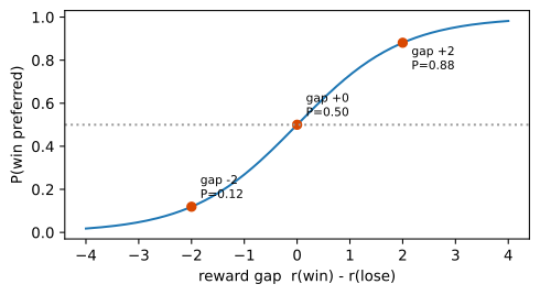
Our reward model is linear in the same three features, r_\phi(y)=\phi^\top f(y), so its learned weights are legible. The gradient of the Bradley–Terry loss for one pair is the feature difference scaled by (\sigma-1) — the familiar logistic form.
# @save
def train_reward_model(rows, steps: int = 300, lr: float = 0.2):
    """Fit a linear Bradley-Terry reward model by gradient descent on @eq-ch07-bt.

    The reward is ``phi . features``; for each pair the gradient pushes the
    weights along the winner-minus-loser feature difference. Because the fit is
    faithful to the labels, a biased annotator produces a biased reward model —
    the learned length weight is the bias made legible.

    Args:
        rows: Preference rows from ``collect_preferences``.
        steps: Full-batch gradient steps.
        lr: Learning rate.

    Returns:
        ``(weights, loss_history)`` with loss at the first, middle, and last step.
    """
    weights = [0.0, 0.0, 0.0]
    history = []
    for step in range(steps):
        gradient = [0.0, 0.0, 0.0]
        loss = 0.0
        for prompt, chosen, rejected, _ in rows:
            delta = [features(prompt, chosen)[i] - features(prompt, rejected)[i] for i in range(3)]
            prob = 1.0 / (1.0 + math.exp(-dot(weights, delta)))
            loss -= math.log(max(prob, 1e-12))
            for i in range(3):
                gradient[i] += (prob - 1.0) * delta[i]
        for i in range(3):
            weights[i] -= lr * gradient[i] / len(rows)
        if step in {0, steps // 2, steps - 1}:
            history.append(loss / len(rows))
    return weights, history
The model fits the comparisons well, and held-out ranking accuracy confirms it generalizes to fresh pairs from the same instrument. But look at the weights.
weights, rm_history = train_reward_model(rows)
task, safety, length = weights
print(f"RM loss: {[round(x, 3) for x in rm_history]}")
print(f"learned weights  task {task:.3f}  safety {safety:.3f}  length {length:+.3f}")
test_rows = collect_preferences(count=200, seed=99)
acc = sum(dot(features(p, c), weights) > dot(features(p, r), weights)
          for p, c, r, _ in test_rows) / len(test_rows)
print(f"held-out ranking accuracy: {acc:.3f}")
RM loss: [0.693, 0.246, 0.235]
learned weights task 1.840 safety 1.840 length +1.718
held-out ranking accuracy: 0.855The length weight is strongly positive even though the product’s specification assigns length a negative weight. That is not a bug in gradient descent; it is an accurate fit to a biased annotator. The controlled version of the audit makes it sharp: give the reward model two answers that are equally correct and equally safe and differ only in length, and it prefers the longer one with probability \sigma(\hat{w}_{\text{length}}\cdot\Delta\text{length}).
delta_length = CANDIDATES[PROMPTS[0]][1][3] - CANDIDATES[PROMPTS[0]][0][3]
print(f"P(reward model prefers the longer of two equally good answers) = "
      f"{1 / (1 + math.exp(-length * delta_length)):.3f}")
P(reward model prefers the longer of two equally good answers) = 0.737This is why reward-model validation must ask which features support a prediction, not only whether it reproduces held-out labels drawn by the same instrument. Held-out accuracy and the length weight are both high, and only one of them is good news. The reward model can read a pooled hidden state of a real sequence classifier, predict several attributes before an explicit aggregation, or parse a generative judge’s decision; Chapter 8 owns outcome-versus-process verifiers and their reasoning-specific robustness. The pairwise loss above describes the sequence-scalar case, and more heads help only when each has reliable labels.
Once r_\phi exists, classic RLHF optimizes the policy against it with reinforcement learning. The objective is expected reward, J(\theta)=\mathbb{E}_{x,\,y\sim\pi_\theta}[r_\phi(x,y)], and because the reward is not differentiable through sampling, the policy gradient moves the derivative onto the log-probability of the sampled response: \nabla_\theta J=\mathbb{E}_{y\sim\pi_\theta}[\,r_\phi(x,y)\,\nabla_\theta\log\pi_\theta(y\mid x)\,]. Sample a response, then push its log-probability up in proportion to its reward. Chapter 23 derives this identity from scratch, subtracts a baseline to cut its variance, and runs REINFORCE on a bandit; we take the result as given. Proximal Policy Optimization (Schulman et al. 2017) wraps it in a clipped surrogate that bounds how far one batch can move the policy, and language-model RLHF adds a leash to a frozen reference:
\max_\theta\;\mathbb{E}_{x,\,y\sim\pi_\theta}[r_\phi(x,y)]-\beta\,\mathbb{E}_{x}\!\left[D_{\mathrm{KL}}\!\left(\pi_\theta(\cdot\mid x)\,\|\,\pi_{\text{ref}}(\cdot\mid x)\right)\right], \tag{7.3}
where D_{\mathrm{KL}} measures how far the policy has departed from the reference \pi_{\text{ref}} (usually the SFT model) and \beta>0 sets the leash. The intent is durable: chase preference reward without discarding the broad behavior the SFT model already has. The operational cost is the moving parts. Figure 7.5 contrasts a classic PPO run — a trainable policy, a frozen reference, a reward model, and usually a value model, fed by a continuous rollout loop — with the offline alternative we build next.
flowchart TB
    SFT["SFT policy +<br/>behavior spec"] --> PAIRS["preference pairs"]
    PAIRS --> RM["Bradley-Terry<br/>reward model"]
    SFT -->|"frozen reference"| PPO
    SFT --> ROLL["current-policy rollouts"]
    ROLL -->|"score fresh responses"| RM
    RM --> PPO["PPO: advantage,<br/>clip, reference KL"]
    PPO -->|"policy samples again"| ROLL
    PAIRS --> DPO["DPO log-ratio loss"]
    SFT -->|"frozen reference"| DPO
    DPO --> OUT(["updated policy,<br/>no rollout loop"])
Learned rewards remain proxies. This chapter measures preference bias and keeps the reference leash; Chapter 8 is the home for Goodhart’s law, reward over-optimization, and verifier exploitation.
7.6 Direct preference optimization
PPO’s apparatus buys on-policy exploration, but if a fixed preference corpus already covers the behavior we want, we can skip the reward model and the rollout loop entirely. Direct Preference Optimization (Rafailov et al. 2023) starts from the same KL-regularized objective of Equation 7.3 and solves it in closed form. The optimal policy is the reference tilted by the exponentiated reward, \pi^*(y\mid x)=\frac{1}{Z(x)}\pi_{\text{ref}}(y\mid x)\exp(r(x,y)/\beta), with Z(x) a prompt-only normalizer. Rearranging for the reward gives r(x,y)=\beta\log\frac{\pi^*(y\mid x)}{\pi_{\text{ref}}(y\mid x)}+\beta\log Z(x). Substitute that into the Bradley–Terry difference of Equation 7.2 and the intractable \beta\log Z(x) term — identical for both completions — cancels. Replacing the unknown optimum with the trainable policy leaves a loss with no reward model in it:
\mathcal{L}_{\text{DPO}}(\theta)=-\mathbb{E}_{(x,y_w,y_l)}\log\sigma\!\left(\beta\left[\log\frac{\pi_\theta(y_w\mid x)}{\pi_{\text{ref}}(y_w\mid x)}-\log\frac{\pi_\theta(y_l\mid x)}{\pi_{\text{ref}}(y_l\mid x)}\right]\right). \tag{7.4}
Every term is operational. The policy log-probability of a response is the sum of its completion-token log-probabilities under the same chat template and response mask we built for SFT — so we already have the machinery. The inner difference asks whether the policy raised the chosen response relative to the reference more than it raised the rejected one; the outer log-sigmoid is binary preference likelihood; \beta sets how far the policy may drift from the reference. We compute the sequence log-probability directly.
# @save
def seq_logp(model, prompt: str, response: str):
    """Summed log-probability of a response's tokens under the chat template.

    This is the quantity inside @eq-ch07-dpo: render the prompt with a
    generation cue, append the response and an end token, and sum the model's
    log-probabilities over exactly the response positions. The reference and
    the policy are scored the same way; their difference is the implicit reward.

    Args:
        model: The model to score under.
        prompt: The user turn.
        response: The candidate assistant response.

    Returns:
        A scalar tensor: the summed completion-token log-probability.
    """
    prompt_ids = render_chat([{"role": "user", "content": prompt}], add_generation_prompt=True)
    full = prompt_ids + tokenizer.encode(response) + [SPECIAL["end"]]
    logp = F.log_softmax(model(torch.tensor([full[:-1]]))[0], dim=-1)[0]
    targets = full[1:]
    start = len(prompt_ids) - 1
    return logp[range(start, len(targets)), targets[start:]].sum()
The training pairs come from the annotator’s own choice. Its length bias makes the longer of two equally-correct answers the chosen one, so DPO on these pairs teaches the model to prefer length — exactly the residual we want to watch propagate. We hold the reference frozen and update a copy of the SFT policy.
# @save
def annotator_best(prompt: str) -> int:
    """Index of the candidate the biased annotator scores highest for a prompt."""
    scores = [dot(features(prompt, i), ANNOTATOR_WEIGHTS) for i in range(len(CANDIDATES[prompt]))]
    return max(range(len(scores)), key=scores.__getitem__)


def dpo_pairs():
    """Build (prompt, chosen, rejected) text pairs from the annotator's preference.

    Chosen is the annotator's top pick — here the longer compliant answer,
    because its length weight tips the balance; rejected is the equally correct
    concise answer. The only systematic difference is length, which isolates
    the bias for @eq-ch07-dpo to absorb.

    Returns:
        A list of ``(prompt, chosen_text, rejected_text)``.
    """
    return [(p, CANDIDATES[p][annotator_best(p)][0], CANDIDATES[p][0][0]) for p in PROMPTS]


def train_dpo(policy, reference, pairs, steps: int = 60, lr: float = 3e-4, beta: float = 0.1):
    """Optimize the DPO loss of @eq-ch07-dpo against a frozen reference.

    Reference log-probabilities are computed once; each step raises the
    implicit-reward margin of chosen over rejected. A gentle step size shifts
    the preference while keeping generation coherent — pushed harder, the same
    loss over-optimizes, which @sec-ch07-dpo demonstrates.

    Args:
        policy: The trainable policy (a copy of the SFT model).
        reference: The frozen SFT reference.
        pairs: ``(prompt, chosen, rejected)`` triples.
        steps: Gradient steps.
        lr: AdamW learning rate.
        beta: The reference-leash strength from @eq-ch07-kl.

    Returns:
        Loss at the first, middle, and last step.
    """
    with torch.no_grad():
        ref = [(seq_logp(reference, p, w).item(), seq_logp(reference, p, l).item()) for p, w, l in pairs]
    optimizer = torch.optim.AdamW(policy.parameters(), lr=lr)
    history = []
    for step in range(steps):
        policy.train()
        loss = 0.0
        for (p, w, l), (ref_w, ref_l) in zip(pairs, ref):
            margin = beta * ((seq_logp(policy, p, w) - ref_w) - (seq_logp(policy, p, l) - ref_l))
            loss = loss - F.logsigmoid(margin)
        loss = loss / len(pairs)
        optimizer.zero_grad(set_to_none=True)
        loss.backward()
        torch.nn.utils.clip_grad_norm_(policy.parameters(), 1.0)
        optimizer.step()
        if step in {0, steps // 2, steps - 1}:
            history.append(loss.item())
    return history
The preference win-rate is the fraction of pairs whose implicit-reward margin favors the chosen (longer) answer. Before training the policy equals the reference, so every margin is exactly zero and the DPO loss starts at \log 2\approx0.693. After training the loss collapses and the policy prefers the longer answer in every pair.
def prefers_longer(policy, reference, pairs, beta: float = 0.1) -> float:
    policy.eval(); reference.eval()
    with torch.no_grad():
        return sum(
            beta * ((seq_logp(policy, p, w) - seq_logp(reference, p, w))
                    - (seq_logp(policy, p, l) - seq_logp(reference, p, l))).item() > 0
            for p, w, l in pairs) / len(pairs)

pairs = dpo_pairs()
reference = ch02.TinyGPT(make_config()); reference.load_state_dict(sft.state_dict())
policy = ch02.TinyGPT(make_config()); policy.load_state_dict(sft.state_dict())
dpo_history = train_dpo(policy, reference, pairs)
print(f"mean chosen length {sum(len(tokenizer.encode(w)) for _, w, _ in pairs) / len(pairs):.1f} tokens"
      f"   mean rejected length {sum(len(tokenizer.encode(l)) for _, _, l in pairs) / len(pairs):.1f}")
print(f"DPO loss: {[round(x, 3) for x in dpo_history]}")
print(f"policy prefers the longer answer in {prefers_longer(policy, reference, pairs):.0%} of pairs")
for user in ("can i get a refund", "how do i reset my password"):
    print(f"  {user!r} -> {chat(policy, user)[0]!r}")
mean chosen length 16.2 tokens mean rejected length 3.8
DPO loss: [0.693, 0.001, 0.0]
policy prefers the longer answer in 100% of pairs
'can i get a refund' -> 'please share your order id and i will check the status.'
'how do i reset my password' -> 'open settings, then security, then reset password.'DPO did exactly what its loss asked: the implicit reward now favors the longer answer everywhere, and at this gentle step size the greedy generations stay coherent. That gap between preference and generation is the senior-level catch — the win-rate can hit 100% while decoding still emits the shorter memorized reply, so preference accuracy and generation quality must be measured separately. Push the same loss harder and the tiny policy over-optimizes: the margin keeps climbing while free generation dissolves into repetition, reward over-optimization in miniature.
overtrained = ch02.TinyGPT(make_config()); overtrained.load_state_dict(sft.state_dict())
train_dpo(overtrained, reference, pairs, lr=1e-3)
print("over-optimized (lr=1e-3):", repr(chat(overtrained, "can i get a refund", max_new=18)[0]))
over-optimized (lr=1e-3): 'wawawawawe e, , , , , , , 'The point is not that DPO is fragile; it is that the length bias we injected at collection has now traveled the whole pipeline. Figure 7.6 tracks one comparable quantity — a preference for the longer answer — from the labels, through the reward model, into the DPO policy.
Show the code that draws this figure
stages = ["labels", "reward model", "DPO policy"]
values = [longer_rate,
          1 / (1 + math.exp(-length * delta_length)),
          prefers_longer(policy, reference, pairs)]
fig, ax = plt.subplots(figsize=(5.4, 3.0))
ax.bar(stages, values, color=["#9ecae1", "#4292c6", "#08519c"])
ax.axhline(0.5, ls="--", color="0.5")
ax.set_ylim(0, 1.05); ax.set_ylabel("P(prefers the longer answer)")
for i, v in enumerate(values):
    ax.text(i, v + 0.02, f"{v:.2f}", ha="center", fontsize=9)
fig.tight_layout()
plt.show()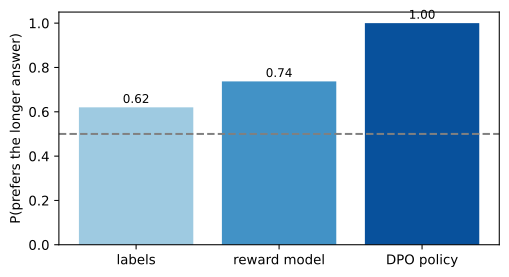
The right response is to repair and re-audit the measurement process — length-matched evaluation slices, length-conditioned preference accuracy, balancing or objective variants chosen from measured product behavior — not to declare that a falling DPO loss certified the specification. DPO also cannot explore: if the corpus came from an older, weaker policy, it holds little information about the current policy’s mistakes, which is the standing argument for online RL when exploration is worth its cost.
NoteIn the interview
Q. Your DPO run reports a preference win-rate of 98% over the SFT reference. Ship it? Not on that number. Win-rate measures the objective DPO optimized, not the product: it rises identically for a policy that learned the intended behavior and one that learned the annotator’s length or position bias. Ask for length-conditioned win-rate and length-matched task quality, the reward or preference source’s audit (position/length rates, swap consistency), and generation-quality evaluation independent of the preference metric. The trap is treating the preference margin as the result; Figure 7.6 is the reason it is only the input.
DPO is one point in a direct-alignment design space — the family of losses that skip the reward model. Each changes one assumption of Equation 7.4.
| Method | Changes vs. DPO | Buys | Main residual |
|---|---|---|---|
| DPO (Rafailov et al. 2023) | — (log-sigmoid of the reference-relative log-ratio) | simple offline preference learning | length bias; needs a reference and paired data |
| IPO (Azar et al. 2024) | squared-loss identity objective, no Bradley–Terry | resists overfitting deterministic preferences | still paired; a tuning target to set |
| KTO (Ethayarajh et al. 2024) | per-example desirable/undesirable labels, not pairs | learns from unpaired thumbs-up/down | prospect-theory assumptions to accept |
| ORPO (Hong et al. 2024) | odds-ratio penalty folded into SFT, no reference | one stage, no frozen copy | couples SFT and preference strength |
| SimPO (Meng et al. 2024) | length-normalized reward, reference-free | drops the reference model; targets length | normalization must match generation length |
Signal, coverage, and operational constraints choose among them; none removes the need to audit the labels. Notice SimPO exists largely to attack the exact length bias we watched travel.
7.7 Scaling feedback: RLAIF and constitutional training
Human comparison is slow and expensive. Reinforcement Learning from AI Feedback (RLAIF) uses a model to produce some preference labels or critiques, usually against an explicit rubric, and feeds them to a reward model or a direct preference loss (Lee et al. 2023). The optimization math does not change because the labeler is a model; the measurement risks do. An AI labeler is cheap, fast, and consistent, and it can also share blind spots with the policy, prefer its own style, follow an instruction injected inside a candidate, or turn a vague rubric into confident but unstable labels. The defenses are the ones we already built plus a few: separate the policy and evaluator contexts, treat candidate text as data rather than instructions, randomize and swap-remap positions, keep human-labeled calibration sets, and stratify agreement by rule. When consequences are high or the rubric is contested, humans stay the authority for the specification and its adjudication.
Constitutional AI is a more structured use of written principles (Bai et al. 2022). A supervised phase has a model critique and revise its own responses against a constitution, producing safer demonstrations; a reinforcement phase then trains on AI-generated preferences under those principles. The durable idea is not a particular list but the traceable transformation written rule → critique → revision or preference → training example → rule-linked evaluation — which is why behavior specifications came first in this chapter. A constitution becomes useful to training only after its conflicts, applicability, and examples are operationalized; natural-language principles do not enforce themselves, and a model-generated critique is evidence to evaluate, not proof of compliance.
The pipeline follows the feedback interface, and the stages compose: SFT for format and demonstrable behavior, preference tuning for subjective comparisons, online RL only where exploration or a verifiable outcome justifies its machinery.
| Available signal | First method to reach for | What it buys | Main residual |
|---|---|---|---|
| Expert can write the target | SFT | simple, stable imitation | weak coverage outside demonstrations |
| Expert can rank fixed candidates | DPO or another direct loss | offline preference learning, no RM/PPO | limited by candidate support and label bias |
| Policy must explore; learned judgment usable | RM + PPO-style RLHF | fresh on-policy data | operational complexity, proxy reward |
| Outcome is programmatically verifiable | online RL with a verifier | scalable objective feedback | verifier gaps (Chapter 8 develops this) |
| Human labels scarce, rubric explicit | RLAIF + human calibration | label scale and consistency | common-mode evaluator bias |
More stages are not automatically better. Every stage earns its place through a held-out, specification-linked delta, or it is complexity without evidence.
7.8 Landscape 2026
Note
Verified 2026-07-20. Hugging Face TRL ships maintained trainers for SFT, reward modeling, DPO, and PPO-family objectives; PEFT and torchtune cover adapter-based and PyTorch-native recipes. Config schemas, default loss normalizations, chat-template handling, and the direct-alignment menu keep changing, and public behavior artifacts evolve — OpenAI maintains a Model Spec, and Anthropic published a revised constitution in early 2026. These are current profiles, not the durable mechanism. Verify live: the TRL, PEFT, and torchtune docs, the OpenAI Model Spec, and Anthropic’s constitution before choosing APIs or adopting any public behavior text. Appendix C owns the annual audit.
7.9 Summary
Post-training turns a next-token predictor into a specified assistant, and its result is decided by the measurement process, not the optimizer. We wrote a behavior rule as data and traced it to its demonstrations, SFT’d Chapter 2’s tiny model into a chat model through a template and a response mask, and showed that masking stops the model from learning to speak the user’s turn. We fit a Bradley–Terry reward model whose learned length weight was the annotator’s bias made legible, then derived DPO from the KL-regularized objective and ran it, watching that same length bias travel from labels to reward model to policy while the preference win-rate hit 100%. The methods follow the signal; Chapter 8 takes reward optimization and its failure modes to reasoning scale.
7.10 Exercises
Derive and check the SFT gradient. For the response-only loss of Equation 7.1 over a softmax head, show that \partial\mathcal{L}/\partial z_j = p_j - \mathbb{1}[j=\text{target}] at a masked position and that masked-out positions contribute zero. Then set
mask_prompt=Falseinsft_train, and predict before running whetherspan_loss(..., "assistant")should change — and explain the number you get.Audit position bias properly. Extend
collect_preferencesto record candidate identities and collect every content pair in both left/right orders. Report the left-choice rate and the swap-consistency (fraction whose verdict survives remapping to identity). Define a release threshold and justify it against the rawleft_ratethe chapter printed.Repair the length bias.
- Build a length-matched evaluation slice from
CANDIDATESand report the reward model’s accuracy on it versus the full held-out set. - Make one intervention in collection (not the loss) that lowers the learned length weight, predict the new weight, then retrain the reward model and check.
- Re-run DPO after your fix and report
prefers_longerand a generation sample together.
- Build a length-matched evaluation slice from
Vary the DPO leash. Sweep
betaandlrintrain_dpoand, for each, record the final loss,prefers_longer, and whetherchat(policy, ...)stays coherent. Identify the regime where the preference margin is fully learned but generation has degraded, and connect it to the over-optimization cell.Turn the reward model into DPO’s target. The chapter fit an explicit reward model and, separately, ran reference-free DPO. Write the value of
beta * (seq_logp(policy) - seq_logp(reference))for the two candidates of one prompt, and explain in what sense DPO is training an implicit reward model — and when you would still want the explicit one.Compare feedback interfaces. For a support behavior of your choice, write one
SpecRule, then construct an SFT demonstration, a preference pair, and a deterministic verifier for it. State what each representation captures and what it loses, and which row of the final decision table it lands on.Defend a pipeline. You have 50,000 fixed human preference pairs from an older policy, a strong SFT checkpoint, no trustworthy online reward service, and a two-week deadline. Choose among SFT-only, DPO, and PPO-based RLHF. Name the evaluation gates, the largest residual risk, and the one measurement that would make you revisit the choice.