A team has enough accelerator time for exactly one base-model run. One proposal is a three-billion-parameter decoder trained on twenty billion tokens; another doubles the parameters and halves the tokens. Both spend nearly the same training compute, and neither states the loss it expects, whether the corpus even contains enough unique text to fill the token budget, or how anyone would notice a bad data mixture before the budget is gone. The decision looks like a modeling choice. It is mostly a measurement problem, and this chapter builds the two instruments that make it measurable.
The first instrument is a scaling law: an empirical surface that predicts loss from model size N and training tokens D. We fit one to a proxy ladder — a handful of tiny models we train ourselves, on real text, in a few seconds — then read the compute-optimal allocation off the fit, attach an honest interval to an extrapolation, and check the compute accounting C \approx 6ND against the runs. The second instrument is the pretraining data pipeline that produces D: we extract an embedded corpus, filter it, catch near-duplicates with MinHash, remove an evaluation plant, sample a source mixture, and measure how many tokens the same sentence costs in different languages. Along the way we watch a base model being evaluated while it trains, and watch a distribution collapse when a model is fed its own output.
Everything here runs at laptop scale, and that is the point. The fitted exponents belong to a nine-kilobyte corpus and an eighty-step budget, not to a frontier model — but the mechanisms are exactly the ones a frontier team uses, and the habit of making an allocation inspectable before it is expensive is the transferable skill. We reuse the byte-pair tokenizer and TinyGPT decoder built in Chapter 2, so nothing about the model is a black box.
5.1 A proxy ladder you can train
The honest way to learn what a scaling law is worth is to fit one to models you trained and can inspect, not to a table of numbers from a paper. So we build a ladder: several TinyGPT models of different sizes, each trained on a different amount of unique text, each evaluated on the same held-out slice. If loss falls smoothly as we climb the ladder, there is a law to fit.
We reuse Chapter 2’s teaching code directly. Its # @save cells were tangled into a module we load here; this is the same tokenizer and model, not a copy.
The corpus is the same nine kilobytes of Alice’s Adventures in Wonderland. We train one tokenizer on it, encode it once, and hold out the last sixth for evaluation — every model on the ladder is scored against this identical, unseen tail.
Two small helpers do the mechanical work. draw samples a batch of aligned next-token windows (the construction from Section 2.2), and heldout_loss averages the model’s cross-entropy over evenly spaced windows of the held-out tail.
BLOCK, BATCH =32, 24def draw(source, generator): starts = torch.randint(0, source.numel() - BLOCK -1, (BATCH,), generator=generator) inputs = torch.stack([source[s : s + BLOCK] for s in starts]) targets = torch.stack([source[s +1 : s + BLOCK +1] for s in starts])return inputs, targets@torch.inference_mode()def heldout_loss(model, source): block = model.config.block_size starts = torch.linspace(0, max(0, source.numel() - block -1), 20).long() losses = []for s in starts: _, loss, _ = model(source[s : s + block].unsqueeze(0), source[s +1 : s + block +1].unsqueeze(0)) losses.append(float(loss))returnfloat(sum(losses) /len(losses))
Now the rung itself. Each rung fixes a model size (width and depth) and a data budget (how many unique leading tokens of the training set it may see), then trains a fixed ten passes over that slice. Varying the unique-token budget is how we move along the data axis honestly: a rung with more unique text is genuinely exposed to more of the language, not merely to the same sentences more times. For N we report non-embedding parameters — the attention and feed-forward weights that actually set model capacity — because a tiny model’s embedding table would otherwise dominate the count and mislabel the axis.
Read the table by column. Down any run of similar D, adding parameters lowers loss — but the effect fades: the largest models on the smallest data budgets barely beat mid-sized ones, because there is not enough unique text to fill their capacity. Down any run of similar N, adding unique tokens lowers loss more reliably. That asymmetry — capacity that goes to waste without data, data that almost always helps — is the entire scaling story in miniature, and the next section makes it a fittable object.
5.2 Power laws you can fit
Language-model loss tends to fall smoothly with resources, and Kaplan and colleagues found the fall is well described by a power law: the reducible part of the loss drops as a resource raised to a negative exponent (Kaplan et al. 2020). For a single resource x,
L(x) = L_\infty + K x^{-\gamma},
\tag{5.1}
where L_\infty is a fitted floor (the loss no amount of this resource removes), K > 0 is a scale, and \gamma > 0 is the exponent. The floor matters: subtract it and take logarithms, and Equation 5.1 becomes a straight line, \log(L - L_\infty) = \log K - \gamma \log x, whose slope is -\gamma. Omit the floor and the “line” bends, and the fitted exponent is wrong. A small \gamma is the sobering case — it means multiplying the resource buys only a sliver of loss.
One resource is not enough, because our ladder varies two. A parameter-only law fitted across runs that also differ in tokens would blame on capacity what was really a difference in exposure. So we fit the joint law Hoffmann and colleagues used (Hoffmann et al. 2022),
L(N, D) = E + A\left(\frac{N}{N_0}\right)^{-\alpha} + B\left(\frac{D}{D_0}\right)^{-\beta},
\tag{5.2}
with a shared floor E, positive coefficients A, B and exponents \alpha, \beta, and fixed reference units N_0, D_0 that only condition the arithmetic and never change a prediction. We hold the fitted law in a small value object whose two methods are the only things we will ask of it: predict a loss, and solve for the best allocation under a compute budget (the second we derive in Section 5.3).
# @saveimport numpy as npfrom dataclasses import dataclassPARAM_REF, TOKEN_REF =1.0e4, 1.0e5# reference units; conditioning only@dataclassclass ScalingLaw:"""A fitted joint law L(N, D) = E + A(N/N0)^-alpha + B(D/D0)^-beta. The five fitted numbers are the whole model of the ladder: ``floor`` is the irreducible loss E, ``param_coeff``/``data_coeff`` scale each resource term, and ``param_exponent``/``data_exponent`` are how fast loss falls with model size and with tokens. Their ratio, not their absolute size, decides how a compute budget should be split between N and D. """ floor: float param_coeff: float data_coeff: float param_exponent: float data_exponent: floatdef loss(self, params, tokens):"""Predict loss for absolute parameter and token counts. Args: params: Non-embedding parameter count(s) N, scalar or array. tokens: Training-token count(s) D, scalar or array. Returns: The predicted cross-entropy under @eq-ch05-joint. """ n = np.asarray(params, dtype=float) / PARAM_REF d = np.asarray(tokens, dtype=float) / TOKEN_REFreturn (self.floor +self.param_coeff * n ** (-self.param_exponent)+self.data_coeff * d ** (-self.data_exponent))def compute_optimal(self, compute):"""Return the loss-minimizing (N, D, loss) on the budget C = 6ND. Args: compute: A training-compute budget C in FLOPs. Returns: A tuple ``(N, D, loss)``: the parameter and token counts that minimize @eq-ch05-joint subject to ``6 * N * D == compute``, and the loss they achieve. The split follows the closed form of @sec-ch05-chinchilla. """ c = compute / (6.0* PARAM_REF * TOKEN_REF) ratio = (self.param_exponent *self.param_coeff) / (self.data_exponent *self.data_coeff) n = (ratio * c **self.data_exponent) ** (1.0/ (self.param_exponent +self.data_exponent)) d = c / nreturn n * PARAM_REF, d * TOKEN_REF, float(self.loss(n * PARAM_REF, d * TOKEN_REF))
The fit itself is least squares in the original loss units, with two guardrails that encode what we know: every coefficient and exponent is kept positive, and the floor is held below the smallest observed loss (a floor above the data would be nonsense). scipy’s curve_fit does the optimization; the bounds keep it in the physically meaningful region.
# @savefrom scipy.optimize import curve_fitdef fit_scaling_law(params, tokens, losses):"""Fit @eq-ch05-joint to measured ladder points by bounded least squares. The fit is done in loss units with positivity bounds on every coefficient and exponent, and the floor E is bounded below the smallest observed loss so the reducible terms explain the *variation* rather than absorbing the floor. Args: params: Sequence of non-embedding parameter counts N. tokens: Sequence of training-token counts D. losses: Sequence of measured losses, one per (N, D). Returns: The fitted :class:`ScalingLaw`. """ n = np.asarray(params, dtype=float) d = np.asarray(tokens, dtype=float) y = np.asarray(losses, dtype=float)def surface(inputs, floor, a, b, alpha, beta): nn, dd = inputsreturn floor + a * (nn / PARAM_REF) ** (-alpha) + b * (dd / TOKEN_REF) ** (-beta) lower = [0.0, 1e-4, 1e-4, 0.02, 0.02] upper = [float(y.min()), 80.0, 80.0, 2.0, 2.0] guess = [float(y.min()) *0.5, 1.0, 1.0, 0.3, 0.3] popt, _ = curve_fit(surface, (n, d), y, p0=guess, bounds=(lower, upper), maxfev=40000)return ScalingLaw(*popt)
We fit it to the ladder and compare each rung’s fitted loss with what we measured.
N = [r["params"] for r in rungs]D = [r["tokens"] for r in rungs]L = [r["loss"] for r in rungs]law = fit_scaling_law(N, D, L)residuals = [obs -float(law.loss(n, d)) for n, d, obs inzip(N, D, L)]print(f"floor E = {law.floor:.3f}")print(f"alpha (N) = {law.param_exponent:.3f} beta (D) = {law.data_exponent:.3f}")print(f"max |residual| over the ladder = {max(abs(r) for r in residuals):.3f} nats")
floor E   = 4.772
alpha (N) = 0.938   beta (D) = 1.390
max |residual| over the ladder = 0.044 nats
Both exponents are positive, so both resources genuinely reduce loss, and the fit tracks every rung to within a few hundredths of a nat. The exponents themselves are far steeper than the frontier values Kaplan reported (near {0.08} for parameters, {0.10} for data) — a nine-kilobyte corpus and an eighty-step budget compress the whole loss range into about half a nat, which inflates the slopes. What transfers is not the number but the ratio, and the ratio is what Section 5.3 turns into an allocation.
An extrapolation is only honest with an interval. We refit the law on residual-resampled copies of the ladder — the residual bootstrap — and read the spread of the extrapolated compute-optimal loss. This interval covers finite-ladder noise; it says nothing about a wrong functional form, an architecture change, or distribution shift, and no bootstrap can.
# @savedef extrapolation_interval(params, tokens, losses, *, multiplier=100.0, samples=120, seed=0):"""Residual-bootstrap the compute-optimal loss at ``multiplier`` times the ladder's largest compute. The point estimate comes from the fit on the real ladder; the interval comes from refitting on residual-resampled copies and taking the 5th/95th percentiles of the extrapolated loss. It quantifies finite-ladder noise only — not model misspecification or distribution shift. Args: params: Sequence of parameter counts N. tokens: Sequence of token counts D. losses: Sequence of measured losses. multiplier: How far past the largest observed compute to extrapolate. samples: Number of bootstrap refits. seed: Seed for the residual resampler. Returns: A dict with the target compute, the compute-optimal ``(opt_params, opt_tokens)``, the point ``loss``, its ``p05``/``p95`` bounds, and the count of ``valid`` bootstrap fits. """ params = np.asarray(params, dtype=float) tokens = np.asarray(tokens, dtype=float) losses = np.asarray(losses, dtype=float) law = fit_scaling_law(params, tokens, losses) target =float((6.0* params * tokens).max() * multiplier) opt_params, opt_tokens, point = law.compute_optimal(target) base = np.asarray(law.loss(params, tokens)) residuals = losses - base residuals = residuals - residuals.mean() rng = np.random.default_rng(seed) draws = []for _ inrange(samples): noisy = base + rng.choice(residuals, size=len(losses))try: _, _, predicted = fit_scaling_law(params, tokens, noisy).compute_optimal(target)exceptException:continueif np.isfinite(predicted): draws.append(predicted +float(rng.choice(residuals))) low, high = np.quantile(draws, (0.05, 0.95))return {"target_compute": target, "opt_params": opt_params, "opt_tokens": opt_tokens,"loss": point, "p05": float(low), "p95": float(high), "valid": len(draws)}
We forecast the compute-optimal loss a hundred times past the ladder’s largest budget, and report its interval.
forecast = extrapolation_interval(N, D, L, multiplier=100.0, samples=120, seed=0)print(f"at 100x the ladder's largest compute (C = {forecast['target_compute']:.2e} FLOPs):")print(f" compute-optimal loss = {forecast['loss']:.3f} "f"[{forecast['p05']:.3f}, {forecast['p95']:.3f}] ({forecast['valid']} valid fits)")
at 100x the ladder's largest compute (C = 1.93e+12 FLOPs):
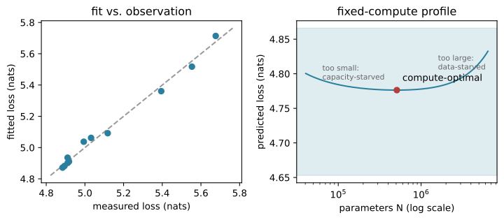
  compute-optimal loss = 4.776 [4.653, 4.866]  (120 valid fits)
Figure 5.1 shows both views: the fit against the observations, and the extrapolated U-curve with its interval.
Show the code that draws this figure
import matplotlib.pyplot as pltfig, (ax1, ax2) = plt.subplots(1, 2, figsize=(7.6, 3.4))fitted = [float(law.loss(n, d)) for n, d inzip(N, D)]ax1.scatter(L, fitted, color="#2a7f9e", zorder=3)lo, hi =min(L + fitted) -0.05, max(L + fitted) +0.05ax1.plot([lo, hi], [lo, hi], "--", color="0.6")ax1.set_xlabel("measured loss (nats)")ax1.set_ylabel("fitted loss (nats)")ax1.set_title("fit vs. observation")target = forecast["target_compute"]n_grid = np.logspace(np.log10(forecast["opt_params"]) -1.1, np.log10(forecast["opt_params"]) +1.1, 200)d_grid = target / (6.0* n_grid)loss_grid = law.loss(n_grid, d_grid)ax2.plot(n_grid, loss_grid, color="#2a7f9e")ax2.axhspan(forecast["p05"], forecast["p95"], color="#2a7f9e", alpha=0.15)ax2.scatter([forecast["opt_params"]], [forecast["loss"]], color="#b13f3f", zorder=3)ax2.annotate("compute-optimal", (forecast["opt_params"], forecast["loss"]), textcoords="offset points", xytext=(6, 10))ax2.annotate("too small:\ncapacity-starved", (n_grid[10], loss_grid[10]), textcoords="offset points", xytext=(8, -2), fontsize=8, color="0.4")ax2.annotate("too large:\ndata-starved", (n_grid[-25], loss_grid[-25]), textcoords="offset points", xytext=(-30, 6), fontsize=8, color="0.4")ax2.set_xscale("log")ax2.set_xlabel("parameters N (log scale)")ax2.set_ylabel("predicted loss (nats)")ax2.set_title("fixed-compute profile")fig.tight_layout()plt.show()
Figure 5.1: Does the fitted law explain the ladder, and what does it predict past it? Left: fitted versus measured loss for the eleven trained rungs (points on the dashed line are perfectly fit). Right: holding compute at 100x the largest rung, loss as a function of how that budget is split; the marked minimum is the compute-optimal model with its residual-bootstrap 90 percent interval. Data are trained locally on nine kilobytes of text.
The right panel’s U is the whole decision. Too far left and the budget is spent re-showing data to a model too small to absorb it; too far right and it buys parameters that never see enough tokens. The minimum belongs to a training objective — Section 5.4 asks whether it is the model you should actually ship.
5.3 Chinchilla makes size and data a joint decision
The U-curve exists because compute is shared between N and D, so we need the exchange rate. For a dense decoder-only Transformer a good first-order estimate — derived in Section 2.7 from the two-FLOPs-per-parameter rule — is
C \approx 6ND,
\tag{5.3}
where C counts training FLOPs, N is non-embedding parameters, and D is tokens seen. The six is a forward pass plus a backward pass that produces gradients for both activations and weights; it is an estimate, not a device invoice, and attention terms, sparsity, and kernel efficiency shift it. Our ladder already reports it in the third column, and it is exact by construction there — which is what lets compute_optimal treat the constraint as an equality. We check that the solver honors it and read three budgets off the fitted law:
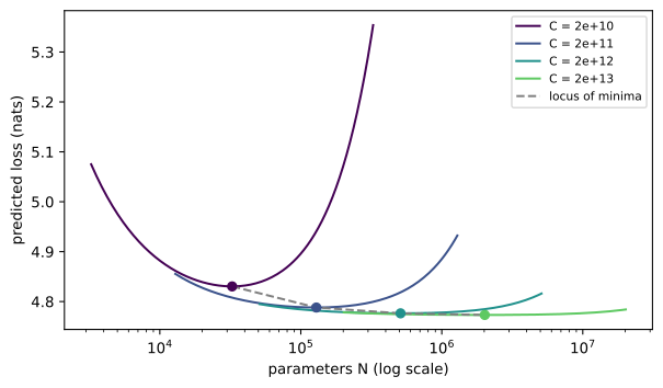
C = 1.93e+10:  N* =    32578  D* =     98954  6ND/C = 1.0000  loss = 4.830
C = 1.93e+11:  N* =   128884  D* =    250123  6ND/C = 1.0000  loss = 4.788
C = 1.93e+12:  N* =   509893  D* =    632227  6ND/C = 1.0000  loss = 4.776
The identity holds to four places, and as compute grows the optimal split shifts. Where does the split come from? Substitute the constraint D = C/(6N) into Equation 5.2 and set the derivative to zero. Writing n = N/N_0, d = D/D_0, and normalized compute c so the constraint is nd = c, we minimize A n^{-\alpha} + B c^{-\beta} n^{\beta}; the stationary point is
The exponents sum to one — every extra unit of compute is divided between the two axes — and their split is set entirely by the ratio of \alpha and \beta. That is the transferable output of the fit, independent of the inflated absolute exponents:
share_N = law.data_exponent / (law.param_exponent + law.data_exponent)share_D = law.param_exponent / (law.param_exponent + law.data_exponent)print(f"N* grows as C^{share_N:.2f}, D* grows as C^{share_D:.2f}")
N* grows as C^0.60, D* grows as C^0.40
Both grow with compute, and roughly together — near the square-root split that makes “grow the model and the data in step” the durable lesson. This is the substance of Chinchilla. Hoffmann and colleagues re-ran the fit at frontier scale and found earlier practice had over-invested in parameters: their 70-billion-parameter Chinchilla, trained on 1.4 trillion tokens, matched the 280-billion-parameter Gopher trained on only 300 billion — four times fewer parameters, far more tokens, better loss (Hoffmann et al. 2022). The single ratio “about twenty tokens per parameter” that people quote from that paper is a consequence of one fitted \alpha/\beta at one scale, not a law of nature; Section 5.4 shows where it stops applying.
Figure 5.2 draws the experiment behind the ratio: fix a compute budget, sweep the split, find the minimum, and repeat at several budgets so the minima trace Equation 5.4.
Show the code that draws this figure
fig, ax = plt.subplots(figsize=(6.4, 3.8))base_compute = (6* np.asarray(N) * np.asarray(D)).max()minima = []for k, mult inenumerate((1, 10, 100, 1000)): budget = base_compute * mult opt_n, _, opt_loss = law.compute_optimal(budget) n_grid = np.logspace(np.log10(opt_n) -1.0, np.log10(opt_n) +1.0, 160) ax.plot(n_grid, law.loss(n_grid, budget / (6.0* n_grid)), color=plt.cm.viridis(k /4), label=f"C = {budget:.0e}") ax.scatter([opt_n], [opt_loss], color=plt.cm.viridis(k /4), zorder=3) minima.append((opt_n, opt_loss))ax.plot([m[0] for m in minima], [m[1] for m in minima], "--", color="0.5", label="locus of minima")ax.set_xscale("log")ax.set_xlabel("parameters N (log scale)")ax.set_ylabel("predicted loss (nats)")ax.legend(fontsize=8)fig.tight_layout()plt.show()
Figure 5.2: Why is there an optimum at every compute budget? Each curve fixes a compute budget and varies the model size along C = 6ND; its minimum (dot) is the compute-optimal model at that budget. The dashed locus through the minima is N* proportional to C^0.6 — the joint law’s allocation rule, drawn from the fit.
A budget is not a schedule until compute becomes wall-clock time. If P_\text{peak} is per-accelerator peak throughput, G the accelerator count, and u the measured model FLOP utilization (MFU) — the fraction of peak the run actually sustains — then t_\text{wall} \approx C / (G\, u\, P_\text{peak}). Using peak throughput silently assumes u = 1, which no real run reaches. The arithmetic is worth doing once with frontier-scale magnitudes, plainly illustrative rather than a quote:
params_7b, tokens_1_4t =7e9, 1.4e12compute_7b =6* params_7b * tokens_1_4taccelerators, peak_flops, mfu =1024, 1.0e15, 0.40# 1024 chips, 1 PFLOP/s each, 40% MFUwall_seconds = compute_7b / (accelerators * mfu * peak_flops)print(f"C = {compute_7b:.2e} FLOPs")print(f"wall time at 40% MFU on 1024 chips = {wall_seconds /86400:.2f} days")print(f"the same run at an optimistic 100% MFU would claim {wall_seconds * mfu /86400:.2f} days")
C = 5.88e+22 FLOPs
wall time at 40% MFU on 1024 chips = 1.66 days
the same run at an optimistic 100% MFU would claim 0.66 days
The MFU term is the difference between a plan and a fantasy: the same FLOPs take two and a half times longer at forty percent than the peak-throughput daydream implies. Chapter 6 owns the execution that determines u; here it is enough to record the FLOP convention and the measured MFU range beside any wall-time estimate.
5.4 Scaling laws are decision tools, not commandments
The compute-optimal model minimizes training loss per unit of training compute. A product also pays inference compute on every request, forever, and that changes the objective. A model served heavily may be worth training past its loss-optimal point — deliberate overtraining — because a smaller model that reaches the same quality is cheaper on every future token. The break-even is a back-of-envelope, and worth seeing concretely (Sardana et al. 2024):
# a Chinchilla-optimal 7B vs a smaller 4B trained on more tokens to match itopt_params_, opt_tokens_ =7e9, 1.4e11over_params, over_tokens =4e9, 8.0e11extra_training =6* over_params * over_tokens -6* opt_params_ * opt_tokens_saving_per_token =2* (opt_params_ - over_params) # ~2N FLOPs per served tokenbreakeven = extra_training / saving_per_tokenprint(f"overtraining costs {extra_training:.2e} extra training FLOPs")print(f"and saves {saving_per_token:.2e} inference FLOPs per served token")print(f"break-even after {breakeven:.2e} served tokens")
overtraining costs 1.33e+22 extra training FLOPs
and saves 6.00e+09 inference FLOPs per served token
break-even after 2.22e+12 served tokens
Past that many served tokens the smaller, overtrained model has repaid its heavier training and keeps saving. That is inference-aware scaling: the training-loss optimum and the deployment-economics optimum are different points, and which one to build depends on how much you will serve. The lesson is not a new ratio to memorize but a habit — run overtraining ladders rather than promoting one number to law.
Other constraints bend the surface in their own ways, and each is its own empirical family, not an add-on to Equation 5.2. When unique data runs short, tokens can be repeated, but the marginal value of a repeat decays — a few epochs help, and beyond roughly four passes extra repetition of the same tokens adds little, so unique tokens and tokens-seen must be tracked separately (Muennighoff et al. 2023). Lower training precision changes effective capacity and can make an overtrained checkpoint more fragile to post-training quantization. Distillation trades a teacher’s cost for a student’s efficiency. Mixture-of-experts models need two laws, one for active compute and one for stored capacity, which is why Chapter 4 separates the two curves. Each deserves its own fit; none is a constant you can carry between architectures.
5.4.1 Apparent emergence
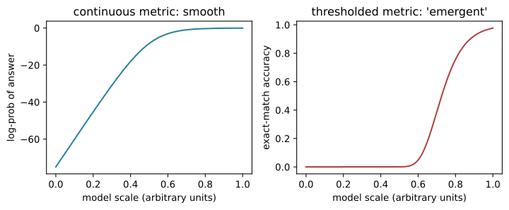
A benchmark curve that is flat and then jumps is often read as an emergent ability appearing at some scale (Wei et al. 2022). Sometimes the capability really does turn on. But the metric can manufacture the jump on its own. Suppose the probability the model assigns to the correct answer rises smoothly with scale. An exact-match score stays at zero until that probability crosses the point where the correct string becomes the single most likely output — and then it snaps up. Schaeffer and colleagues showed that swapping the discontinuous metric for a continuous one (answer log-probability, partial credit) often turns the “emergence” back into a smooth curve (Schaeffer et al. 2023). Figure 5.3 makes the illusion concrete: one smooth quantity, two ways of reading it.
Figure 5.3: Is an ability emerging, or is the metric discretizing a smooth trend? Both panels share the same underlying per-token success probability rising smoothly with scale. Left: mean log-probability of the correct answer — smooth. Right: exact-match accuracy on a 12-token answer, which needs every token right, so it stays near zero then snaps up. Nothing discontinuous happened to the model.
The operational response is not to deny thresholds but to keep continuous observables — answer log-likelihood, margin over alternatives, calibration, partial credit — beside any headline accuracy, so a launch gate can stay discrete while the learning curve stays diagnosable. And pretraining compute is no longer the only axis: reinforcement-learning compute (Chapter 8, Chapter 23) and test-time compute buy quality after the base run. Keep those ledgers separate before optimizing the portfolio.
NoteIn the interview
Q. You fit a scaling law and it says the compute-optimal model is 7B on 140B tokens. Is that the model you ship? Not necessarily. Chinchilla-optimality minimizes loss per unit of training compute; a served product also pays inference on every request for the model’s whole life. If you will serve a lot, a smaller model trained well past its loss-optimal point is usually cheaper over its lifetime, even though it costs more to train. The trap is quoting “twenty tokens per parameter” as a universal constant — it is one fitted ratio at one scale, and it ignores inference entirely.
5.5 Base-model evaluation while the run is alive
A base model is a next-token predictor, not a chat product, and evaluating it through a chat wrapper confounds pretraining quality with templates, sampling, and post-training. The first instrument is the training objective itself. For target tokens x_1,\dots,x_T,
the mean negative log-likelihood, and perplexity is its exponential — an effective branching factor. But a single aggregate number hides where a model is weak. We take the largest model on our ladder and measure its loss on slices instead of in bulk:
from torch.nn import functional as Fbig =max(rungs, key=lambda r: r["params"])["model"]@torch.inference_mode()def slice_loss(text): ids = torch.tensor(tokenizer.encode(text), dtype=torch.long) block = big.config.block_sizeif ids.numel() < block +1: _, loss, _ = big(ids[:-1].unsqueeze(0), ids[1:].unsqueeze(0))returnfloat(loss) starts = torch.linspace(0, ids.numel() - block -1, 12).long()returnfloat(np.mean([float(big(ids[s:s+block].unsqueeze(0), ids[s+1:s+block+1].unsqueeze(0))[1])for s in starts]))print(f"English (held-out Alice) : {slice_loss(tokenizer.decode(heldout.tolist())):.3f}")print(f"Spanish sentence : {slice_loss('Una ingeniera mide los tokens antes de fijar el presupuesto del proyecto.'):.3f}")print(f"Arabic sentence : {slice_loss('يقيس المهندس الدقيق الرموز قبل تحديد الميزانية النهائية للمشروع.'):.3f}")
The Arabic loss is far above the English one: our English-trained tokenizer shatters Arabic into byte fragments the model has never modeled in context, and a per-slice view exposes that immediately where an aggregate would bury it. The Spanish number is the subtle trap — it can sit below the in-distribution English tail, not because the model knows Spanish, but because per-token cross-entropy is not comparable across texts with different token densities. Comparing perplexities is only valid under one tokenizer, normalization, and document policy; across tokenizers you need a byte or character denominator (bits per byte). Fertility, in Section 5.8, is the same fact seen from the cost side.
The second instrument scores candidate answers by conditional log-likelihood rather than sampling one and hoping decoding noise is representative. For a prompt q and candidate completion a,
'The Queen said' + ' off with' -> -4.511
'The Queen said' + ' nothing'  -> -4.951
'The Queen said' + ' qzx'      -> -6.688
The mechanism works: the model scores the Wonderland-idiomatic ” off with” highest and the gibberish ” qzx” lowest, cleanly separating fluent continuations from noise. It is honest about its limits, too — a model this small, trained on nine kilobytes, cannot resolve fine semantic distinctions, and its rankings are weak evidence of capability, not proof of it. That is exactly why base evaluation is telemetry, not a verdict: in-flight evaluation runs while training continues and asks whether optimization is healthy and the mixture is producing the intended capabilities. A useful checkpoint contract logs held-out and per-slice cross-entropy at exact token counts, gradient and update norms, non-finite counters, a small pinned set of conditional-likelihood tasks, and the residual between observed loss and the scaling-law prediction at the current N, D, C — enough to reconstruct every number and to alert on a trajectory (a residual growing across checkpoints) rather than one threshold. Chapter 22 supplies the statistical machinery; this section supplies its base-model inputs.
5.6 Data is a governed supply chain
Every number so far assumed we had D tokens to spend. But D is not the size of a folder. It is what survives acquisition, extraction, an eligibility policy, filtering, deduplication, mixture sampling, and repetition — and reporting “three trillion tokens” without naming the stage and the tokenizer is close to meaningless. A corpus ledger has to distinguish at least the stages in Figure 5.4, because the count drops at every gate and repetition can push the last one back up.
flowchart LR
    A["raw bytes<br/>(crawled archive)"] --> B["extracted<br/>documents"]
    B --> C["eligible<br/>(rights + quality)"]
    C --> D["near-unique<br/>(deduplicated)"]
    D --> E["mixture<br/>(sampled quotas)"]
    E --> F["tokens seen<br/>(× repeats)"]
Figure 5.4: Why is D not the size of a folder? Each gate discards tokens, so a token count is ambiguous until it names its stage — and the final stage can exceed the one before it because repetition re-counts the same tokens. A quoted ‘token count’ without a stage hides which of these numbers it means.
Common Crawl makes the stages concrete: WARC stores raw responses, WAT stores computed metadata, and WET stores extracted plaintext — convenient but already stripped of structure and carrying someone’s extraction decisions. We keep provenance from the start, in a record whose six fields exist because policy needs every one of them. Extraction turns raw records into these documents and assigns each a stable identifier.
# @saveimport hashlib, refrom dataclasses import dataclass as _dataclassWORD = re.compile(r"\w+", re.UNICODE)@_dataclass(frozen=True)class Document:"""One extracted record with the provenance a policy decision needs. ``source`` and ``rights`` are kept distinct on purpose: a crawler being able to fetch a page (source) is not the same as a license to train on it (rights), and collapsing them into a single ``safe`` flag is how corpora quietly admit text they had no right to. """ doc_id: str url: str source: str language: str rights: str text: strdef extract_records(raw_records):"""Turn raw crawl records into :class:`Document` values with stable IDs. Args: raw_records: Iterable of dicts with ``url``, ``source``, ``rights``, ``lang``, and ``text`` keys (the fields a WET record and its headers supply). Returns: A list of :class:`Document`, one per record, each ``doc_id`` a short hash of the URL so the same page always extracts to the same identifier. """ documents = []for record in raw_records: doc_id = hashlib.sha1(record["url"].encode()).hexdigest()[:10] documents.append(Document(doc_id, record["url"], record["source"], record["lang"], record["rights"], record["text"].strip()))return documents
Our embedded corpus is a handful of records built to exercise the pipeline: clean reference and library and community documents, a planted near-duplicate of one reference page (same body, an extra footer line), a document carrying a benchmark answer, a restricted-rights copy, commercial spam, and a one-line stub. All of them share a boilerplate navigation bar, so the deduplicator will have to tell real duplication from shared furniture.
def nav():return"Home About Login Cart Help"body_ref = ("The archive preserves a checked statement about the river survey. ""Editors record each source and keep the wording plain and legible. ""The measured level rose after the spring melt and receded by autumn. ") *3body_lib = ("A library record describes the botany of alpine meadows in plain prose. ""Roots, leaves, and seeds are cataloged with dates and collector initials. ""The herbarium sheet notes elevation, slope, and the surrounding tree line. ") *3body_com = ("A community thread discusses tuning a small telescope for planetary views. ""Members compare eyepieces, focal ratios, and the seeing on humid nights. ""One post records aperture and magnification against a stable star field. ") *3raw = [ {"url": "https://ref.example/a", "source": "reference", "rights": "licensed", "lang": "en", "text": nav() +"\n"+ body_ref}, {"url": "https://ref.example/a-mirror", "source": "reference", "rights": "licensed", "lang": "en", "text": nav() +"\n"+ body_ref +"\nUpdated: minor footer revision."}, {"url": "https://lib.example/b", "source": "library", "rights": "public-domain", "lang": "en", "text": nav() +"\n"+ body_lib}, {"url": "https://com.example/c", "source": "community", "rights": "permission", "lang": "en", "text": nav() +"\n"+ body_com}, {"url": "https://ref.example/d", "source": "reference", "rights": "licensed", "lang": "en", "text": "The benchmark secret answer is cobalt river. "*6+ body_ref}, {"url": "https://ref.example/e", "source": "reference", "rights": "restricted", "lang": "en", "text": body_ref}, {"url": "https://spam.example/f", "source": "web", "rights": "licensed", "lang": "en", "text": "\n".join(["BUY NOW CLICK HERE LIMITED OFFER"] *40)}, {"url": "https://short.example/g", "source": "community", "rights": "permission", "lang": "en", "text": "Short notice."},]for i inrange(3): raw.append({"url": f"https://ref.example/r{i}", "source": "reference", "rights": "licensed", "lang": "en","text": nav() +f"\nReference note {i}. "+"A durable checked record with plain readable prose about surveys and dates. "*6})for i inrange(2): raw.append({"url": f"https://lib.example/l{i}", "source": "library", "rights": "public-domain", "lang": "en","text": nav() +f"\nLibrary note {i}. "+"A durable public-domain record cataloged with dates and provenance. "*6})raw.append({"url": "https://com.example/c2", "source": "community", "rights": "permission", "lang": "en","text": nav() +"\n"+"A second community record comparing methods and instruments in plain prose. "*7})documents = extract_records(raw)first = documents[0]print(f"extracted {len(documents)} documents")print(f"trace: id={first.doc_id} source={first.source} rights={first.rights} lang={first.language}")print(f" url={first.url}")
Every admitted token should trace back through this record to a source, a transformation history, a policy decision, and a reproducible text hash. That lineage does not settle the legal question of whether a document may be trained on — rights vary by jurisdiction and contract, and the AI data commons is contracting as publishers withdraw permission (Longpre et al. 2024) — but it makes the organization’s decision inspectable and, when a source must be removed, lets you find every descendant: the extracts, the synthetic transforms, the mixtures, the checkpoints. Chapter 18 owns deletion in agent memory; the lineage principle starts at acquisition.
5.7 Filter, deduplicate, decontaminate
Extraction maximizes recall; curation decides what should actually train the model. Three operations do different jobs and should write different reason codes. A filter scores or rejects individual documents. Deduplication finds repeated content within and across sources. Decontamination removes training candidates that overlap evaluation material. We build them in that order.
Early corpora such as C4 filtered with transparent heuristics — language, length, character ratios, repetition, blocked terms (Raffel et al. 2020) — which are cheap and debuggable but encode cultural assumptions; the C4 audit found identity-term blocklists removed disproportionately many documents about and by minority groups. Learned quality classifiers (used by FineWeb-Edu and others) rank documents by a trained notion of quality (Penedo et al. 2024), but the label source is a policy choice, and an evaluator’s preferences can hide behind a score. Our filter stays transparent on purpose: rights, length, alphabetic ratio, and line repetition, each an inspectable feature.
# @savefrom collections import Counter, defaultdict@_dataclass(frozen=True)class FilterPolicy:"""Auditable thresholds for a transparent quality filter. Each field is a single interpretable knob so a rejection can always be explained by one named reason rather than an opaque score. """ allowed_rights: tuple= ("licensed", "public-domain", "permission") min_words: int=40 min_alpha_ratio: float=0.55 max_repeated_line_fraction: float=0.5def document_features(text):"""Measure interpretable surface features without treating them as truth. Args: text: The document body. Returns: A tuple ``(word_count, alpha_ratio, repeated_line_fraction)`` — the three quantities the filter thresholds. """ words = WORD.findall(text) visible = [c for c in text ifnot c.isspace()] lines = [ln.strip() for ln in text.splitlines() if ln.strip()] repeated =0.0ifnot lines else1.0-len(set(lines)) /len(lines) alpha =sum(c.isalpha() for c in visible) /max(1, len(visible))returnlen(words), alpha, repeateddef filter_documents(documents, policy=FilterPolicy()):"""Apply rights and quality gates, recording a reason for each rejection. Args: documents: Iterable of :class:`Document`. policy: The :class:`FilterPolicy` thresholds to apply. Returns: A tuple ``(kept, rejected)`` where ``rejected`` items are ``{doc_id, reason}`` dicts, so the drop at this gate is always explainable. """ kept, rejected = [], []for doc in documents: words, alpha, repeated = document_features(doc.text) reason =Noneif doc.rights notin policy.allowed_rights: reason ="rights"elif words < policy.min_words: reason ="too-short"elif alpha < policy.min_alpha_ratio: reason ="low-alpha"elif repeated > policy.max_repeated_line_fraction: reason ="repetition"if reason isNone: kept.append(doc)else: rejected.append({"doc_id": doc.doc_id, "reason": reason})return kept, rejected
We run it on the extracted corpus and count what survived and why.
eligible, rejected = filter_documents(documents)print(f"kept {len(eligible)} of {len(documents)}; rejections: {dict(Counter(r['reason'] for r in rejected))}")
The gate removed the restricted-rights copy, the one-line stub, and the commercial spam (on line repetition), each with a named reason rather than a silent disappearance. Now deduplication, which is where the interesting mechanics live.
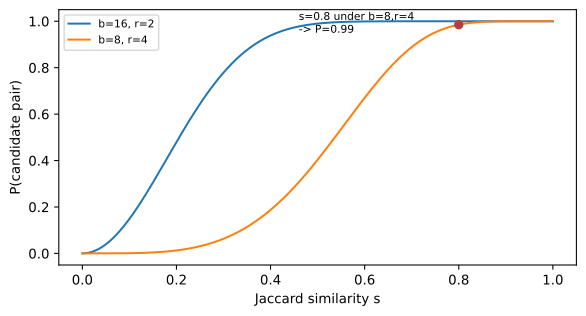
Exact hashing only catches byte-identical records; web duplicates differ by a menu, a timestamp, or one inserted line. So we compare sets of word shingles — overlapping five-word sequences — with the Jaccard similarity J(A,B) = |A \cap B| / |A \cup B|. Comparing all pairs is quadratic, so we approximate. A MinHash signature records, for each of several hash functions, the minimum hashed shingle; two documents agree on one component with probability equal to their Jaccard similarity. Locality-sensitive hashing then splits the signature into b bands of r rows and calls a pair a candidate if any band matches, with probability
More bands raise recall (and false positives); more rows per band sharpen the threshold. We build the pieces — shingles, similarity, a signature — then the deduplicator that uses LSH only to propose candidates and confirms each with an exact Jaccard check before merging clusters with union-find (Lee et al. 2022).
# @savedef word_shingles(text, width=5, cap=200):"""Return a bounded set of hashed word shingles for a document. Args: text: The document body. width: Shingle length in words (5 is a common choice). cap: Keep only the ``cap`` lowest-hashing shingles (bottom-k sampling), so long and short documents get comparable-size signatures. Returns: A set of shingle strings. """ words = WORD.findall(text.casefold()) shingles = {" ".join(words[i:i + width]) for i inrange(max(1, len(words) - width +1))}returnset(sorted(shingles, key=lambda s: hashlib.blake2b(s.encode(), digest_size=8).digest())[:cap])def jaccard(a, b):"""Return the Jaccard similarity of two shingle sets."""returnlen(a & b) /max(1, len(a | b))def minhash_signature(shingles, permutations=32, prime=(1<<61) -1):"""Return a MinHash signature whose agreement rate estimates Jaccard. Args: shingles: A set of shingle strings. permutations: Signature length; more permutations sharpen the estimate. prime: Modulus for the (a*h + b) mod p hash family. Returns: A tuple of ``permutations`` minima, one per hash function. """ifnot shingles:return (0,) * permutations hashed = [int.from_bytes(hashlib.blake2b(s.encode(), digest_size=8).digest(), "big") for s in shingles]returntuple(min(((2* k +1) * h +2654435761* (k +1)) % prime for h in hashed)for k inrange(permutations))
# @savedef near_deduplicate(documents, threshold=0.7, permutations=32, bands=16):"""Cluster near-duplicate documents and keep one exemplar from each cluster. LSH proposes candidate pairs from shared signature bands; each candidate is confirmed by an exact Jaccard check above ``threshold`` before its documents are merged with union-find. The longest document in a cluster is kept, so boilerplate that is merely *shared* across otherwise-distinct documents does not collapse them. Args: documents: Iterable of :class:`Document`. threshold: Minimum confirmed Jaccard similarity to merge a pair. permutations: MinHash signature length. bands: Number of LSH bands; ``permutations`` must divide evenly by it. Returns: A tuple ``(kept, clusters)`` where ``kept`` is the surviving documents in input order and ``clusters`` lists each cluster's member IDs. """ docs =list(documents) shingles = [word_shingles(d.text) for d in docs] signatures = [minhash_signature(s, permutations) for s in shingles] parent =list(range(len(docs)))def find(i):while parent[i] != i: parent[i] = parent[parent[i]] i = parent[i]return idef union(i, j): ri, rj = find(i), find(j)if ri != rj: parent[max(ri, rj)] =min(ri, rj) width = permutations // bands buckets = defaultdict(list)for i, sig inenumerate(signatures):for band inrange(bands): buckets[(band, sig[band * width:(band +1) * width])].append(i) candidates =set()for members in buckets.values():for x inrange(len(members)):for y inrange(x +1, len(members)): candidates.add((members[x], members[y]))for i, j insorted(candidates):if jaccard(shingles[i], shingles[j]) >= threshold: union(i, j) clusters = defaultdict(list)for i inrange(len(docs)): clusters[find(i)].append(i) kept =sorted(max(members, key=lambda i: (len(docs[i].text), -i)) for members in clusters.values())return [docs[i] for i in kept], [[docs[i].doc_id for i in members] for members in clusters.values()]
We run it on the eligible documents and inspect which clusters merged.
deduped, clusters = near_deduplicate(eligible)print(f"{len(eligible)} -> {len(deduped)} after near-deduplication")print("clusters with more than one member:", [c for c in clusters iflen(c) >1])
11 -> 10 after near-deduplication
clusters with more than one member: [['2ac722ddcf', 'fb29afe755']]
The deduplicator collapsed exactly the planted pair — the reference page and its footer-revised mirror — into one document, while the library, community, and reference notes that share the same navigation bar all survived, because bottom-k shingling and the confirmation step distinguish a shared header from a shared body. Figure 5.5 shows why the band parameters, not the threshold alone, set what counts as a duplicate.
Figure 5.5: How do the band parameters turn a similarity into a match probability? Each curve is P(candidate | s) = 1 - (1 - sr)b for one (bands, rows) setting. Raising rows per band moves the knee right and sharpens it — the same similarity can be a near-certain match under one setting and a coin flip under another, which is why b and r are the real threshold, not a single cutoff.
Finally decontamination, a different question: does a training candidate contain evaluation material? We normalize whitespace and case and drop any document that contains a known evaluation string. Production systems combine substrings, n-grams, canaries, and cautious semantic matching, and recheck synthetic descendants — but the principle is visible in the small version.
# @savedef decontaminate(documents, evaluation_strings, min_chars=20):"""Remove documents containing a normalized evaluation substring. Args: documents: Iterable of :class:`Document`. evaluation_strings: Known evaluation prompts/answers to exclude. min_chars: Ignore needles shorter than this after normalization, so trivially short strings do not match everything. Returns: A tuple ``(kept, removed)`` where ``removed`` items are ``{doc_id}`` dicts — the documents pulled for touching the evaluation set. """def normalize(text):return" ".join(WORD.findall(text.casefold())) needles = [normalize(s) for s in evaluation_strings iflen(normalize(s)) >= min_chars] kept, removed = [], []for doc in documents: body = normalize(doc.text)ifany(needle in body for needle in needles): removed.append({"doc_id": doc.doc_id})else: kept.append(doc)return kept, removed
We give it the one evaluation string we planted and watch the offending document leave.
clean, removed = decontaminate(deduped, ["benchmark secret answer is cobalt river"])print(f"{len(deduped)} -> {len(clean)} after decontamination; removed {[r['doc_id'] for r in removed]}")
10 -> 9 after decontamination; removed ['5a1d54655b']
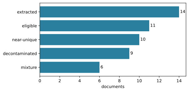
The planted benchmark document is gone, and Figure 5.6 counts the survivors through every gate. A one-time decontamination pass is necessary but not sufficient: a benchmark discovered in the corpus after the run means the score is contaminated, not that the data is retroactively clean, and any synthetic rephrasing of a leaked example must be rechecked.
Show the code that draws this figure
mixture_size =6stages = ["extracted", "eligible", "near-unique", "decontaminated", "mixture"]counts = [len(documents), len(eligible), len(deduped), len(clean), mixture_size]fig, ax = plt.subplots(figsize=(6.4, 3.2))ax.barh(range(len(stages)), counts, color="#2a7f9e")for i, c inenumerate(counts): ax.text(c +0.1, i, str(c), va="center")ax.set_yticks(range(len(stages)))ax.set_yticklabels(stages)ax.invert_yaxis()ax.set_xlabel("documents")fig.tight_layout()plt.show()
Figure 5.6: How many documents survive each gate? The real counts from our pipeline: extraction admits everything, the rights-and-quality filter and near-deduplication and decontamination each remove some, and the sampled mixture selects a fixed quota. The drop is evidence a gate acted — it is not, by itself, evidence of quality; the reason ledger is.
5.8 Mixtures, fertility, and curriculum
A curated corpus is still not a training distribution until source weights are chosen. Sampling in proportion to available tokens just reproduces crawl abundance, which over-weights repetitive commercial pages and lets scarce, high-value books or low-resource languages vanish. Mixture weights are model hyperparameters with governance consequences, so we convert weights into exact document quotas and refuse to silently backfill a missing source from leftovers.
# @saveimport mathdef mix_documents(documents, weights, total):"""Select an exact per-source quota from documents by target weights. Weights are turned into integer quotas by the largest-remainder method, and a zero-weight source contributes nothing — the mixture never quietly fills a shortfall from another source, so the realized proportions are inspectable. Args: documents: Iterable of :class:`Document`. weights: Mapping from source name to non-negative weight. total: Total documents to select. Returns: The selected documents, grouped by source in name order. """ positive = {s: w for s, w in weights.items() if w >0} eligible = [d for d in documents if d.source in positive] total_weight =sum(positive.values()) exact = {s: total * w / total_weight for s, w in positive.items()} quota = {s: math.floor(v) for s, v in exact.items()}for s insorted(positive, key=lambda s: -(exact[s] - quota[s])):ifsum(quota.values()) >= total:break quota[s] +=1 pools = defaultdict(list)for d insorted(eligible, key=lambda d: d.doc_id): pools[d.source].append(d) selected = []for s insorted(quota): selected.extend(pools[s][:quota[s]])return selected
We ask for a 50/30/20 reference-library-community split of six documents, with web weighted to zero.
mixture = mix_documents(clean, {"reference": 0.5, "library": 0.3, "community": 0.2, "web": 0.0}, total=6)print("mixture by source:", dict(Counter(d.source for d in mixture)))
mixture by source: {'community': 1, 'library': 2, 'reference': 3}
The realized mixture is exactly the requested 50/30/20 split across reference, library, and community, and the zero-weight web source contributes nothing. Choosing those weights well is its own research problem: DoReMi trains a small proxy model to find weights that minimize worst-case excess loss across domains, then trains the real model on them (Xie et al. 2023); RegMix trains many small proxies on sampled mixtures and fits a regression from weights to downstream score (Liu et al. 2024). Both replace intuition with experiments, and both inherit a transfer question — proxy rankings can change with scale — so candidate weights must be validated at more than one budget. The public corpus lineage is best read the same way, as methodological progress rather than a size leaderboard: C4’s single-snapshot heuristic cleanup, the Pile’s named-domain mixture, RedPajama’s and Dolma’s reproducible transforms and released tooling, and DCLM’s and FineWeb’s controlled ablations each added named sources, reproducible transformations, quality signals, and then controlled comparisons — in that order. A raw token count without that provenance says almost nothing.
Weights decide which tokens; fertility decides how many each language costs. Chapter 2’s byte-fallback tokenizer can encode any Unicode string, but coverage is not efficiency. Fertility is the number of tokens per character, and a language’s token allocation is D_\ell = f_\ell Q_\ell for character count Q_\ell and fertility f_\ell(Ahia et al. 2023). We measure it directly on the same tokenizer.
# @savedef measure_fertility(samples, encode):"""Measure tokenizer fertility (tokens per character) per language sample. Args: samples: Mapping from language name to a sample string. encode: A tokenizer's ``encode`` function returning a token-ID list. Returns: A list of ``{language, characters, tokens, tokens_per_char}`` dicts, one per sample — the per-character cost the same content incurs. """ rows = []for language, text in samples.items(): tokens =len(encode(text)) rows.append({"language": language, "characters": len(text), "tokens": tokens,"tokens_per_char": tokens /max(1, len(text))})return rows
We encode the same sentence in four languages with Chapter 2’s tokenizer and read off the per-character cost.
sentence = {"English": "A careful engineer measures tokens before fixing a budget.","Spanish": "Una ingeniera cuidadosa mide los tokens antes de fijar el presupuesto.","Arabic": "يقيس المهندس الدقيق الرموز قبل تحديد الميزانية.","Hindi": "एक सावधान इंजीनियर बजट तय करने से पहले टोकन मापता है।"}for row in measure_fertility(sentence, tokenizer.encode):print(f"{row['language']:8}{row['tokens']:3d} tokens / {row['characters']:3d} chars "f"= {row['tokens_per_char']:.2f} tokens/char")
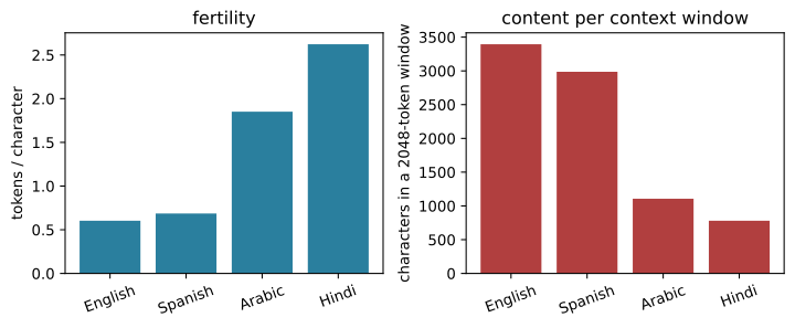
The equity problem is now a number. Our English-leaning tokenizer spends about four times as many tokens per character on Hindi as on English and roughly three times as many on Arabic. Figure 5.7 turns that into context-window content: at equal fertility every language would fit the same amount of meaning in a fixed window, but a high-fertility language gets a fraction of it — and pays proportionally more to train and serve.
Show the code that draws this figure
rows = measure_fertility(sentence, tokenizer.encode)langs = [r["language"] for r in rows]fert = [r["tokens_per_char"] for r in rows]chars_per_window = [2048/ f for f in fert]fig, (axl, axr) = plt.subplots(1, 2, figsize=(7.6, 3.2))axl.bar(langs, fert, color="#2a7f9e")axl.set_ylabel("tokens / character")axl.set_title("fertility")axr.bar(langs, chars_per_window, color="#b13f3f")axr.set_ylabel("characters in a 2048-token window")axr.set_title("content per context window")for ax in (axl, axr): ax.tick_params(axis="x", rotation=20)fig.tight_layout()plt.show()
Figure 5.7: What does tokenizer fertility cost a language? Left: tokens per character for the same sentence under Chapter 2’s English-trained BPE. Right: how many characters of each language fit in a fixed 2048-token window — the high-fertility languages get far less content per context and pay more per character to train and serve. These are toy measurements of one small tokenizer, not a language benchmark.
The response to high fertility is not to down-weight the language, which only saves tokens by withholding content; it is to retrain the shared tokenizer on representative text, allocate more tokens, or use byte-aware architectures — and to make that choice before the major run, because changing the tokenizer breaks perplexity comparisons and checkpoint compatibility. Curation and mixing also stage over time. Mid-training keeps a language-model objective while shifting data quality, domains, or sequence lengths; continued pretraining resumes from a checkpoint on a new distribution; annealing lowers the learning rate toward zero and is an optimizer intervention, not a synonym for high-quality data. A common program runs broad pretraining, then a capability-targeted mixture, then a long-context stage with genuinely long documents — and Chapter 3 owns the positional machinery that long context needs, while Chapter 11 owns customization after a base model exists.
5.9 Synthetic data at the data wall
Unique, high-quality tokens in a target distribution are finite, and “the data wall” names the point where they run short. Synthetic data is the tempting answer, but the phrase hides four mechanisms with different failure modes: a grounded transformation of a real document (summary, rephrasing) that keeps its parent; fresh generation from prompts or simulators; verified generation accepted only after an executable or human check; and recursive self-consumption, where model output replaces the real distribution across generations. The first three can help — rephrasing real web text and mixing it with the original improves efficiency (Maini et al. 2024). The fourth is where model collapse lives.
Shumailov and colleagues showed that indiscriminate recursive replacement loses the tails of a distribution and eventually distorts it: rare modes are sampled less often, so they appear even less often in the next generation, and the support narrows (Shumailov et al. 2024). Gerstgrasser and colleagues found the crucial qualifier — accumulating generated data alongside the original real data avoided collapse in their settings, where pure replacement did not (Gerstgrasser et al. 2024). We can watch both happen with a one-dimensional toy: each generation fits a Gaussian to the current data (a deliberately lossy model) and samples a new dataset, either replacing the old data or keeping the real anchor. Because a finite sample slightly under-estimates spread, replacement compounds that shrinkage generation over generation, while the real anchor keeps re-injecting the tails. We average over many seeds so the systematic trend, not one random walk, is what we read.
# @savedef recursive_generations(generations=8, sample_size=20, mode="replace", seed=0):"""Simulate one lineage of a distribution learned from its own samples. Each generation fits a Gaussian (maximum-likelihood mean and spread) to the current data and draws a fresh sample from it. Under ``"replace"`` the fresh sample becomes the next generation's data; under ``"accumulate"`` it is pooled with the original real data before resampling, so the real tails keep returning. Args: generations: Number of generations to simulate. sample_size: Points per generation (small sizes collapse faster). mode: ``"replace"`` or ``"accumulate"``. seed: Seed for the generator. Returns: A tuple ``(spread_by_generation, final_sample)``: the standard deviation after each generation and the final generation's samples. """ rng = np.random.default_rng(seed) real = rng.normal(0.0, 1.0, sample_size) data = real.copy() spread = [float(data.std())]for _ inrange(generations): fresh = rng.normal(data.mean(), data.std(), sample_size) data = fresh if mode =="replace"else rng.choice(np.concatenate([real, fresh]), sample_size, replace=False) spread.append(float(data.std()))return spread, data
We run both modes over two hundred lineages and average the spread trajectory so the systematic trend, not one random walk, is what we read.
seeds =range(200)replace = np.mean([recursive_generations(mode="replace", seed=s)[0] for s in seeds], axis=0)accumulate = np.mean([recursive_generations(mode="accumulate", seed=s)[0] for s in seeds], axis=0)print("spread by generation (mean over 200 lineages):")print(" replace ", [f"{x:.2f}"for x in replace])print(" accumulate", [f"{x:.2f}"for x in accumulate])
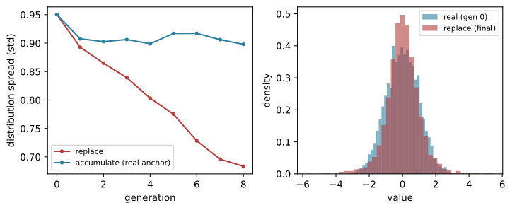
Under replacement the spread decays monotonically — the distribution is collapsing toward a point — while accumulation holds it near its starting value. Figure 5.8 shows the trajectories and the narrowing tail directly.
Show the code that draws this figure
final_replace = np.concatenate([recursive_generations(mode="replace", seed=s)[1] for s in seeds])gen0 = np.concatenate([recursive_generations(generations=0, mode="replace", seed=s)[1] for s in seeds])fig, (axl, axr) = plt.subplots(1, 2, figsize=(7.6, 3.2))axl.plot(range(len(replace)), replace, "-o", color="#b13f3f", label="replace", markersize=3)axl.plot(range(len(accumulate)), accumulate, "-o", color="#2a7f9e", label="accumulate (real anchor)", markersize=3)axl.set_xlabel("generation")axl.set_ylabel("distribution spread (std)")axl.legend(fontsize=8)axr.hist(gen0, bins=40, alpha=0.6, color="#2a7f9e", label="real (gen 0)", density=True)axr.hist(final_replace, bins=40, alpha=0.6, color="#b13f3f", label="replace (final)", density=True)axr.set_xlabel("value")axr.set_ylabel("density")axr.legend(fontsize=8)fig.tight_layout()plt.show()
Figure 5.8: What does recursive self-consumption do to a distribution? Left: the spread of the learned distribution across generations, averaged over 200 lineages — replacement decays toward a point, while accumulating the real data alongside the synthetic holds it steady. Right: pooled final-generation samples under replacement have visibly narrower tails than the original real data. Collapse is a loss of tails, not of the mean.
The engineering rule is not a universal synthetic percentage but an authentic anchor: keep an immutable, provenance-tagged slice of the real target distribution, compare real-only, synthetic-only, and mixed conditions at equal compute, and track tail slices and diversity, not just average loss. Verification changes the failure rather than removing it — an executable test validates code strongly, but a learned judge tends to reward its own preferences and becomes both a ceiling and a bias source. Synthetic data is most defensible when it supplies a known missing intervention — worked examples, rare failure cases, executable programs — and least defensible when a generator fills a volume quota with average loss as the only guardrail.
5.10 Landscape 2026
The durable spine above — fit multiple ways, hold out runs, report uncertainty, keep provenance, evaluate on immutable slices — outlasts any particular corpus or ratio. The examples below are current compositions of those mechanisms, not recipes.
Note
Verify live: 2026-07-19. Staged base-model programs are the current norm: the OLMo 3 technical report describes broad pretraining of several trillion tokens, a mid-training stage, and model-size-dependent long-context stages, with microanneals that compare a candidate source plus web text against a compute-matched web-only control before promotion. A 2026 analysis of IsoFLOP fitting reports that the common parabolic fit can be biased by finite runs and noise — reinforcing the durable action of fitting several ways and holding out runs. Reinforcement-learning and test-time compute are now treated as additional scaling axes (quarantined here to Chapters 8 and 23), and the evidence contradicts any “pretraining is over” slogan: acquisition, mixture search, mid-training, and synthetic-data verification remain active engineering. Verify these specifics against primary sources before relying on them.
5.11 Summary
We built two instruments and connected them. A proxy ladder of tiny models, trained on real text, gave measured loss across many sizes and token budgets; a bounded least-squares fit turned it into a joint law whose exponent ratio — not its inflated absolute values — sets the compute-optimal split, which we derived, checked against C \approx 6ND, and extrapolated with a residual-bootstrap interval. On the data side we ran the pipeline that produces D: extract, filter, MinHash-deduplicate (catching a plant), decontaminate, and mix by exact quota, then measured multilingual fertility and watched a distribution collapse under recursive self-consumption. Chapter 6 turns this budget and data manifest into a real training run.
5.12 Exercises
Stress the extrapolation. Refit the law after dropping the two largest-compute rungs, then predict the original 100x target. Compare the point estimate and interval with the full-ladder forecast, and explain how much of the change came from extrapolation reach versus the smaller ladder.
Price two allocations. Using the fitted law, compute the compute-optimal token count for a hypothetical 3-billion-parameter model, then for a 10x-overtrained allocation of the same model. Convert both to FLOPs with Equation 5.3 and to accelerator-days with a stated MFU, and say which costs your estimate omits.
Expose filter bias. Add a rare-language slice to the embedded corpus, then design a filter that raises the average quality score while deleting most of that slice. (a) Quantify retention and per-language token counts before and after. (b) Propose a gate that makes the deletion visible without forcing every domain to identical statistics.
Break the deduplicator. Raise bands to 32 in near_deduplicate (so rows per band drop) and re-run on the corpus. Does the planted near-duplicate still merge? Use Equation 5.7 to explain the change, then find a (bands, threshold) pair that keeps the plant merged but stops merging two documents that share only the navigation bar.
Measure contamination inflation. Insert one cloze answer from Section 5.5 into a controlled fraction of the training slice, skip decontamination, retrain the largest rung, and measure how candidate_score and held-out loss change as the contaminated fraction rises. Distinguish memorization from genuine improvement.
Tune the collapse demo. In recursive_generations, sweep sample_size over {10, 20, 40, 80} for the replace mode. (a) Plot the final-generation spread against sample size. (b) Explain why larger samples collapse more slowly, and relate it to why a frontier corpus needs a large authentic anchor rather than a fixed synthetic percentage.
Design a mid-training curriculum. Propose three base-model stages for a code assistant. For each, specify the source mixture, unique versus repeated tokens, sequence-length distribution, the learning-rate intervention, the control branch, and the promotion metric — and justify why each stage belongs before post-training.
Ahia, Orevaoghene, Sachin Kumar, Hila Gonen, et al. 2023. “Do All Languages Cost the Same? Tokenization in the Era of Commercial Language Models.”Proceedings of the 2023 Conference on Empirical Methods in Natural Language Processing.
Gerstgrasser, Matthias, Rylan Schaeffer, Apratim Dey, et al. 2024. “Is Model Collapse Inevitable? Breaking the Curse of Recursion by Accumulating Real and Synthetic Data.”arXiv Preprint arXiv:2404.01413.
Hoffmann, Jordan et al. 2022. “Training Compute-Optimal Large Language Models.”Advances in Neural Information Processing Systems.
Kaplan, Jared et al. 2020. “Scaling Laws for Neural Language Models.”arXiv Preprint arXiv:2001.08361.
Lee, Katherine, Daphne Ippolito, Andrew Nystrom, et al. 2022. “Deduplicating Training Data Makes Language Models Better.”Proceedings of the 60th Annual Meeting of the Association for Computational Linguistics.
Liu, Qian, Xiaosen Zheng, Niklas Muennighoff, et al. 2024. “RegMix: Data Mixture as Regression for Language Model Pre-Training.”arXiv Preprint arXiv:2407.01492.
Longpre, Shayne, Robert Mahari, Ariel Lee, et al. 2024. “Consent in Crisis: The Rapid Decline of the AI Data Commons.”arXiv Preprint arXiv:2407.14933.
Maini, Pratyush, Skyler Seto, He Bai, et al. 2024. “Rephrasing the Web: A Recipe for Compute and Data-Efficient Language Modeling.”arXiv Preprint arXiv:2401.16380.
Muennighoff, Niklas, Alexander M. Rush, Boaz Barak, et al. 2023. “Scaling Data-Constrained Language Models.”Advances in Neural Information Processing Systems.
Penedo, Guilherme, Hynek Kydlı́ček, Anton Lozhkov, et al. 2024. “The FineWeb Datasets: Decanting the Web for the Finest Text Data at Scale.”arXiv Preprint arXiv:2406.17557.
Raffel, Colin, Noam Shazeer, Adam Roberts, et al. 2020. “Exploring the Limits of Transfer Learning with a Unified Text-to-Text Transformer.”Journal of Machine Learning Research 21.
Sardana, Nikhil, Jacob Portes, Sasha Doubov, and Jonathan Frankle. 2024. “Beyond Chinchilla-Optimal: Accounting for Inference in Language Model Scaling Laws.”International Conference on Machine Learning.
Schaeffer, Rylan, Brando Miranda, and Sanmi Koyejo. 2023. “Are Emergent Abilities of Large Language Models a Mirage?”Advances in Neural Information Processing Systems.
Shumailov, Ilia, Zakhar Shumaylov, Yiren Zhao, Nicolas Papernot, Ross Anderson, and Yarin Gal. 2024. “AI Models Collapse When Trained on Recursively Generated Data.”Nature 631: 755–59.
Wei, Jason, Yi Tay, Rishi Bommasani, Colin Raffel, et al. 2022. “Emergent Abilities of Large Language Models.”Transactions on Machine Learning Research.
Xie, Sang Michael, Hieu Pham, Xuanyi Dong, et al. 2023. “DoReMi: Optimizing Data Mixtures Speeds up Language Model Pretraining.”Advances in Neural Information Processing Systems.