We are now ready to build a complete GPT from scratch and train it while we read. Chapter 1 treated the model as a served endpoint that maps context to a continuation; this chapter opens the box and implements everything inside that endpoint, in small executed steps: (i) a byte-pair tokenizer trained on our own corpus; (ii) scaled dot-product attention, derived rather than asserted; (iii) the causal mask that keeps the future out of the past; (iv) multi-head attention, the feed-forward block, and the residual stream that ties them together; (v) the full decoder-only model with a tied language-model head; (vi) a training loop — AdamW, a warmup-cosine schedule — whose loss curve and generated samples we read honestly; and (vii) cached generation, whose speed and memory we measure rather than estimate.
The corpus is nine kilobytes of Alice’s Adventures in Wonderland — public domain, small enough to embed in the book’s repository, and real English rather than synthetic filler. The model is about 140,000 parameters and trains in seconds on a CPU, which means every number and every generated string on these pages is produced live when the book is built. That is the point of working at toy scale: nothing is hidden, everything is checkable, and the mechanisms are exactly the ones running inside a frontier model — only the constants change. Implementing the pieces ourselves, once, is the cheapest insurance we can buy against every later chapter: serving (Chapter 10), long context (Chapter 3), and interpretability (Chapter 25) all assume the picture we build here.
2.1 A byte-pair tokenizer
A neural network consumes integers, not strings. The tokenizer defines the mapping between them, and that mapping fixes more than convenience: it determines the rows of the embedding table, the columns of the output head, and the unit in which context, cost, and throughput are measured. In Section 1.2 we trained a toy character-pair encoder to see why frequent strings become cheap; here we build the real thing — a byte-level BPE tokenizer of the kind production models actually freeze and ship (Sennrich et al. 2016).
We start from the corpus. It is the opening of Alice’s Adventures in Wonderland (Carroll, 1865), sliced to just over nine kilobytes and stored under data/ch02/.
from pathlib import Pathcorpus = Path("data/ch02/alice.txt").read_text(encoding="utf-8")print(f"{len(corpus)} characters, {len(corpus.encode('utf-8'))} UTF-8 bytes")print(corpus[:193])
9186 characters, 9368 UTF-8 bytes
Alice was beginning to get very tired of sitting by her sister on the bank, and of having nothing to do: once or twice she had peeped into the book her sister was reading, but it had no picture
Note the two counts differ: the text contains curly quotation marks, and UTF-8 encodes each of those as three bytes. That detail decides our base vocabulary. If we started from characters we would need an inventory of every character we might ever meet — an open-ended set. If we start from bytes, the base vocabulary is exactly the 256 possible byte values, and every string in every language already has an encoding before we learn anything. There is no unknown-token case, ever. Byte-pair encoding then makes common strings cheaper: it repeatedly finds the most frequent adjacent pair of tokens and merges it into a new token. We record each learned rule in a small immutable value.
# @savefrom dataclasses import dataclass@dataclass(frozen=True)class Merge:"""One learned BPE rule: the adjacent pair (left, right) becomes new_id. Merges are the entire learned state of a BPE tokenizer. Applied in training order they encode text; expanded recursively they decode it. """ left: int right: int new_id: intdef _merge_pair(ids: list[int], pair: tuple[int, int], new_id: int) ->list[int]:"""Replace every non-overlapping occurrence of pair with new_id.""" merged: list[int] = [] index =0while index <len(ids):if index +1<len(ids) and (ids[index], ids[index +1]) == pair: merged.append(new_id) index +=2else: merged.append(ids[index]) index +=1return merged
The tokenizer itself holds the merge list and the byte expansion of every token ID. Training is a loop: count adjacent pairs, pick the most frequent (with a deterministic tie-break, so two runs always learn the same vocabulary), rewrite the stream, repeat until the vocabulary reaches the requested size.
# @savefrom collections import Counterclass BytePairTokenizer:"""A byte-level BPE tokenizer: 256 byte tokens plus learned merges. Because the base vocabulary is every possible byte, any Unicode string encodes without an unknown-token path — unfamiliar text simply falls back to more, smaller tokens. The vocabulary is fixed the moment training stops; a model trained on top of it inherits that freeze. """def__init__(self, merges: list[Merge] |None=None) ->None:self.merges =list(merges or [])self.token_bytes = {index: bytes([index]) for index inrange(256)}for merge inself.merges:self.token_bytes[merge.new_id] = (self.token_bytes[merge.left] +self.token_bytes[merge.right] )@propertydef vocab_size(self) ->int:"""Return the fixed number of token IDs this tokenizer recognizes."""return256+len(self.merges)@classmethoddef train(cls, text: str, vocab_size: int) ->"BytePairTokenizer":"""Learn merges from UTF-8 text until the vocabulary reaches vocab_size. Args: text: Training text; it determines merge order and nothing else. vocab_size: Target vocabulary size, at least 256. Returns: A tokenizer with up to ``vocab_size - 256`` learned merges. Raises: ValueError: If vocab_size would not retain all 256 byte tokens. """if vocab_size <256:raiseValueError("vocab_size must retain all 256 byte tokens") ids =list(text.encode("utf-8")) tokenizer = cls()for new_id inrange(256, vocab_size): counts = Counter(zip(ids, ids[1:]))ifnot counts:break pair =min(counts, key=lambda item: (-counts[item], item)) ids = _merge_pair(ids, pair, new_id) tokenizer.merges.append(Merge(*pair, new_id)) tokenizer.token_bytes[new_id] = ( tokenizer.token_bytes[pair[0]] + tokenizer.token_bytes[pair[1]] )return tokenizerdef encode(self, text: str) ->list[int]:"""Encode any Unicode string by replaying the learned merges in order. Args: text: Text to encode as UTF-8 bytes plus merges. Returns: Token IDs, every one below ``vocab_size``. """ ids =list(text.encode("utf-8"))for merge inself.merges: ids = _merge_pair(ids, (merge.left, merge.right), merge.new_id)return idsdef decode(self, ids: list[int], errors: str="strict") ->str:"""Expand token IDs to bytes and decode the result as UTF-8. Args: ids: Token IDs produced by ``encode`` (or by a model). errors: UTF-8 error policy; a sampling model can emit byte sequences that are not valid UTF-8, so generation uses ``"replace"`` while round-trip checks keep ``"strict"``. Returns: The reconstructed string. """returnb"".join(self.token_bytes[index] for index in ids).decode("utf-8", errors=errors )
We train it on the corpus, asking for a vocabulary of 512 — the 256 bytes plus 256 learned merges — and look at what it learned first.
tokenizer = BytePairTokenizer.train(corpus, vocab_size=512)print(f"vocab_size = {tokenizer.vocab_size}")for merge in tokenizer.merges[:8]: left, right = tokenizer.token_bytes[merge.left], tokenizer.token_bytes[merge.right]print(f" id {merge.new_id}: {left!r} + {right!r} -> {tokenizer.token_bytes[merge.new_id]!r}")
vocab_size = 512
  id 256: b'e' + b' ' -> b'e '
  id 257: b' ' + b't' -> b' t'
  id 258: b't' + b' ' -> b't '
  id 259: b'e' + b'r' -> b'er'
  id 260: b' t' + b'h' -> b' th'
  id 261: b'i' + b'n' -> b'in'
  id 262: b' ' + b'a' -> b' a'
  id 263: b' ' + b's' -> b' s'
The first merges are exactly what frequency predicts: e followed by space, th, spaced articles. Later merges build on earlier ones, so whole common words condense into single IDs. Encoding replays this history; decoding expands it back to the original bytes. We check the round trip on a string the tokenizer has never seen, including an emoji that exists nowhere in the corpus.
probe ="Alice waited by the rabbit-hole 🐇"ids = tokenizer.encode(probe)print(f"{len(probe.encode('utf-8'))} bytes -> {len(ids)} tokens")print("ids:", ids)print("round trip exact:", tokenizer.decode(ids) == probe)
The familiar words compress to single high-numbered IDs, while the emoji falls back to its four raw bytes (the IDs below 256 at the end) — inefficient but never unrepresentable. That asymmetry is called fertility: the same byte count costs different token counts depending on how well the tokenizer’s training distribution matches the input. Chapter 5 measures fertility across languages at pretraining scale. On its own corpus, the tokenizer earns its keep:
One consequence deserves stating before we build the model on top: the tokenizer is now frozen. The model we are about to construct will have an embedding table with exactly 512 rows and an output layer with exactly 512 columns. Adding a merge later would create a row and a column no gradient has ever touched. You can always encode new text — the byte fallback guarantees it — but you cannot change the vocabulary without surgery on the model itself. Tokenization is part of the architecture, not a request-time utility.
2.2 The next-token objective
What should the model do with these token streams? A language model assigns probability to sequences. The probability chain rule factorizes any joint distribution over a sequence x_{1:T}=(x_1,\ldots,x_T) into one conditional per position:
where \theta is the set of all model parameters. A causal language model implements the right-hand side directly: one network that, given a prefix, outputs a distribution over the next token. Nothing about Equation 2.1 is an approximation — the factorization is exact for any distribution. The modeling assumption is only that one network with shared weights can represent every conditional.
Training pairs each prefix with the token that actually followed it. From one contiguous token stream we can manufacture an aligned example at every position: the input at position t is x_t, and the label is x_{t+1}. This is teacher forcing — during training every prefix comes from the real text, never from the model’s own (initially terrible) predictions. The alignment is easiest to trust after seeing it once with real IDs:
Every row is one training example, and an input window of T tokens yields T of them at once. The helper that draws such windows from a stream is four lines of indexing, and it is worth reading closely because an off-by-one here is the classic way to leak labels:
# @saveimport torchdef next_token_batch( data: torch.Tensor, block_size: int, batch_size: int, generator: torch.Generator,) ->tuple[torch.Tensor, torch.Tensor]:"""Draw aligned (input, target) windows from one contiguous token stream. Targets are the same window shifted one position later, so position t of the input is paired with the token that actually followed it. Every position in the window is a training example. Args: data: A 1-D tensor holding the encoded token stream. block_size: Window length T; each example predicts T next tokens. batch_size: Number of windows to draw. generator: Seeded generator choosing the window start offsets. Returns: A tuple ``(inputs, targets)``, each shaped ``(batch_size, block_size)``. """ starts = torch.randint(0, data.numel() - block_size -1, (batch_size,), generator=generator ) inputs = torch.stack([data[start : start + block_size] for start in starts]) targets = torch.stack([data[start +1 : start + block_size +1] for start in starts])return inputs, targets
The model will emit a logit for every vocabulary item at every position; softmax turns each row of logits into a distribution, and the loss is the mean negative log probability of the true next token:
for a batch of B windows of length T. This is cross-entropy, and it rewards exactly one thing: putting probability mass on the observed next token. It does not reward truthfulness, helpfulness, or task completion — those arrive, to the extent they do, through data and through the post-training of Chapter 7. Perplexity is \exp(\mathcal{L}), readable as an effective branching factor among tokens.
The objective also hands us a free diagnostic. Before any training, a sanely initialized model spreads probability almost uniformly, so its loss should sit near -\log(1/V)=\ln V. For our V=512 that is \ln 512 = 6.24. When we first run the assembled model later in this chapter, we will check its initial loss against this number — if it starts much lower, something (usually the mask or the target alignment) is letting the label leak into the input.
2.3 Scaled dot-product attention
The model must turn “a prefix of tokens” into “a prediction at each position”, and the hard part is letting position t use relevant earlier positions, where relevance depends on content. A convolution sees a fixed neighborhood. A recurrent state compresses the whole prefix into one vector updated in order. Attention takes a third route: every position performs a learned lookup over all visible positions (Vaswani et al. 2017).
The intuition has three roles. Each position publishes a query — a vector describing what it is looking for. Each position also publishes a key — a vector advertising what it can offer — and a value — the actual information it will hand over if selected. A query is compared against every key; positions whose keys match the query contribute their values, in proportion to the match. Queries ask, keys advertise, values deliver.
Formally, let X\in\mathbb{R}^{T\times d} hold one d-dimensional vector per position. Learned projection matrices produce the three roles, Q=XW_Q, K=XW_K, V=XW_V, each row a d_k-dimensional vector, and one attention output row is a weighted average of value rows:
where A\in\mathbb{R}^{T\times T} holds the attention weights (A_{ij} is how much position i draws from position j), softmax is applied to each row, and d_k is the width of each query and key. Every symbol except the \sqrt{d_k} is forced by the intuition: dot products measure query-key match, softmax turns scores into a positive, sum-to-one mixture, and the matrix product AV takes the mixture of values.
So why divide by \sqrt{d_k}? Because dot products grow with dimension. If query and key components are roughly independent with unit variance, their dot product is a sum of d_k terms and its standard deviation is about \sqrt{d_k}. We can watch this happen:
The measured standard deviation tracks \sqrt{d_k} almost exactly, and dividing by it restores scale 1.0 at every width. The reason we care is what large scores do to softmax. Feed it scores at the spread a width-256 head would produce unscaled, and the distribution collapses:
torch.set_printoptions(precision=2, sci_mode=False)scores = torch.randn(6, generator=torch.Generator().manual_seed(1))print("softmax at score scale 2:", torch.softmax(scores *2, -1))print("softmax at score scale 16:", torch.softmax(scores *16, -1))
At scale 16 nearly all mass sits on two entries and the rest are zero to two decimal places. A saturated softmax passes almost no gradient to the losing positions, so the model cannot learn to redistribute its attention. The \sqrt{d_k} keeps scores in softmax’s responsive range regardless of head width. That is the entire derivation — Equation 2.3 is the intuition plus one variance correction.
The implementation is Equation 2.3 line for line, returning the weights as well as the output so we can inspect them:
# @saveimport mathdef scaled_dot_product_attention( query: torch.Tensor, key: torch.Tensor, value: torch.Tensor, mask: torch.Tensor |None=None,) ->tuple[torch.Tensor, torch.Tensor]:"""Compute attention outputs and weights for one set of projections. Scores are query-key dot products scaled by sqrt(d_k) so their spread stays inside softmax's responsive range at any head width; each output row is the weight-averaged mixture of value rows. Args: query: Queries shaped ``(..., T_q, d_k)``. key: Keys shaped ``(..., T_k, d_k)``. value: Values shaped ``(..., T_k, d_v)``. mask: Optional boolean tensor broadcastable to ``(..., T_q, T_k)``; True marks pairs that must receive zero weight. Returns: A tuple ``(output, weights)`` shaped ``(..., T_q, d_v)`` and ``(..., T_q, T_k)``; each weight row is non-negative and sums to 1. """ scores = query @ key.transpose(-2, -1) / math.sqrt(query.size(-1))if mask isnotNone: scores = scores.masked_fill(mask, float("-inf")) weights = scores.softmax(dim=-1)return weights @ value, weights
To see it produce something interpretable, we run a four-token example small enough to check by hand. Pretend the sequence is “The rabbit was late” and that the projections have already been learned. We write the query, key, and value rows ourselves, with a story: the query of “was” is looking for its subject, and the key of “rabbit” advertises “I am a noun”. Values are one-hot so that each position’s payload is recognizable in the output.
Read the weight matrix one row at a time, since each row is one position’s lookup. Row 0, “The”, has a zero query — it asks for nothing — and gets the uniform mixture 0.25 everywhere: attention with no preference is an average. Row 2, “was”, is the sharp one: its query aligns with the key of “rabbit” and takes 0.97 of the weight, so its output is essentially the value of “rabbit” — the lookup found the subject. Row 3, “late”, splits its attention: 0.68 on “rabbit” and 0.25 on “was”, a soft mixture of two relevant positions rather than a hard choice. And because we chose one-hot values, each output row is its weight row — a reminder that attention’s output is never anything more exotic than a weighted average of value vectors.
One thing about this matrix should bother you: row 0 draws weight from columns 1, 2, and 3 — positions that come later in the sequence. For a model trained to predict the next token, that is not a quirk; it is a fatal bug, and it is the next section’s problem.
NoteIn the interview
Q. Why does attention divide by \sqrt{d_k} and not, say, d_k? The dot product of two roughly independent unit-variance vectors has standard deviation \sqrt{d_k}, so dividing by \sqrt{d_k} restores spread 1.0 at any head width; dividing by d_k would crush scores toward zero and flatten every attention pattern toward uniform. The trap is answering “it stabilizes training” without the variance argument — the interviewer wants the one-line derivation, and it is the difference between recalling the formula and owning it.
2.4 Multi-head attention and the causal mask
First, the bug. A team trains its first language model and the loss collapses within a few hundred steps to near zero, while generated text stays incoherent. The architecture has no causal mask: at position t, attention can read position t+1 — which is, by the teacher-forcing construction of Section 2.2, the exact label the model is being scored on. The optimizer discovers the shortcut immediately. The loss is real arithmetic attached to an invalid information path, and every downstream number the run produced is worthless. The fix is the causal mask: position t may attend to positions {1} through t and to nothing later. In Equation 2.3 this means forcing A_{ij}=0 whenever j>i, which we achieve by setting those scores to -\infty before the softmax — an exponentiated -\infty contributes zero mass. Applied to the worked example:
The upper triangle is exactly zero — those lookups no longer exist. Row 0 now has nowhere to look but itself, so its weight is 1.0 there; row 2 still finds “rabbit”, because its subject sits safely in the past. Each row renormalizes over what remains visible. The mask costs nothing to apply and is the single most important line in the model: with it, all T positions can be trained in parallel on one window (each position sees precisely its own prefix) and generation cannot cheat because there is nothing ahead to read.
The second upgrade is capacity. One attention map imposes one notion of relevance per layer: a single softmax over the prefix must simultaneously serve “find my subject”, “find the matching quotation mark”, and “copy the previous token”. Multi-head attention runs H independent lookups in parallel, each in a subspace of width d_h=d/H, then concatenates the H outputs and mixes them with a final projection W_O. The heads are not separate networks — they are slices of the same three projected tensors, computed in one batched matrix multiply. With that, plus two practical details, we can write the layer we will actually use. The details: we normalize queries and keys per head before the dot product (QK normalization, an RMS rescaling that keeps score magnitudes controlled over a long training run), and we accept an optional cache of past keys and values — idle until the final section, where it becomes the entire story.
# @savefrom torch import Tensor, nnLayerCache =tuple[Tensor, Tensor]@dataclass(frozen=True)class GPTConfig:"""Hyperparameters that fix every tensor shape in the model. vocab_size ties the model to one frozen tokenizer; block_size caps how many positions the model can represent at once; d_model is the width of the residual stream; n_heads splits attention into d_model // n_heads subspaces; n_layers stacks identical blocks; mlp_ratio sizes the feed-forward hidden width relative to d_model. """ vocab_size: int block_size: int=128 d_model: int=64 n_heads: int=4 n_layers: int=2 mlp_ratio: float=8/3
# @saveclass CausalSelfAttention(nn.Module):"""Masked multi-head attention over a token sequence, cache-ready. One linear layer projects the input to queries, keys, and values for all heads at once; heads are views of that tensor, not separate modules. Masking compares absolute key positions with absolute query positions, so the same code is correct whether the layer sees a full window (training) or one new token extending a cache (generation). """def__init__(self, config: GPTConfig) ->None:super().__init__()if config.d_model % config.n_heads:raiseValueError("d_model must be divisible by n_heads")self.n_heads = config.n_headsself.head_dim = config.d_model // config.n_headsself.qkv = nn.Linear(config.d_model, 3* config.d_model, bias=False)self.q_norm = nn.RMSNorm(self.head_dim)self.k_norm = nn.RMSNorm(self.head_dim)self.output = nn.Linear(config.d_model, config.d_model, bias=False)def forward(self, x: Tensor, past: LayerCache |None=None) ->tuple[Tensor, LayerCache]: batch, steps, width = x.shape qkv =self.qkv(x).view(batch, steps, 3, self.n_heads, self.head_dim) query, key, value = qkv.permute(2, 0, 3, 1, 4).unbind(0) query, key =self.q_norm(query), self.k_norm(key) past_steps =0if past isNoneelse past[0].size(-2)if past isnotNone: key = torch.cat((past[0], key), dim=-2) value = torch.cat((past[1], value), dim=-2) scores = query @ key.transpose(-2, -1) / math.sqrt(self.head_dim) query_positions = past_steps + torch.arange(steps, device=x.device)[:, None] key_positions = torch.arange(key.size(-2), device=x.device)[None, :] scores = scores.masked_fill(key_positions > query_positions, float("-inf")) mixed = scores.softmax(dim=-1) @ value mixed = mixed.transpose(1, 2).contiguous().view(batch, steps, width)returnself.output(mixed), (key, value)
A shape trace confirms the plumbing: a batch of 2 sequences of 6 positions at width 64 goes in, the same shape comes out, and the returned cache holds one key and one value tensor per head per position.
And the property that matters more than any shape — the mask actually seals the future. We change the last position’s input and check that every earlier output is bit-for-bit unchanged:
Zero — not small, zero. Information from position 6 has no path into positions 1 through 5. This is the executable form of the causal contract, and the chapter’s test suite pins it permanently.
2.5 The residual stream and the transformer block
Attention moves information between positions. It is deliberately bad at transforming it: the output is a weighted average of linearly projected inputs. The transformer pairs it with a second sublayer, a position-wise feed-forward network (FFN), that does the opposite — a genuine nonlinear transformation applied to each position independently, with no communication at all. The architecture alternates the two, and the way they compose is the most useful mental picture in the book: the residual stream.
Each position carries a width-d vector from the embedding all the way to the output. No sublayer ever replaces that vector. Instead each sublayer reads the stream, computes an update, and adds it back:
The plus signs carry the meaning. Gradients flow through the identity path untouched, which is what lets deep stacks train; and semantically, the stream becomes a shared bus into which every sublayer writes and from which every later sublayer reads. Chapter 25 builds its interpretability toolkit on exactly this picture — asking what each component reads from the stream and what direction it writes back. Figure 2.1 draws one block.
flowchart LR
    X["residual stream X(l)"] --> N1["RMSNorm"]
    N1 --> A["causal multi-head attention<br/>(mixes across positions)"]
    A --> P1(("+"))
    X --> P1
    P1 --> H["X(l + 1/2)"]
    H --> N2["RMSNorm"]
    N2 --> F["SwiGLU FFN<br/>(each position independently)"]
    F --> P2(("+"))
    H --> P2
    P2 --> Y["residual stream X(l+1)"]
Figure 2.1: How does one block update the residual stream? Both sublayers read a normalized copy and add their update back; attention is the only place positions communicate, and the FFN transforms each position independently.
Two design choices in Equation 2.4 are worth naming because they differ from the 2017 original. Normalization happens before each sublayer (pre-norm), which keeps the identity path clean and trains stably at depth, and the statistic is RMSNorm — a rescaling by root-mean-square without mean subtraction, which does LayerNorm’s stabilizing job with less work (Zhang and Sennrich 2019). The FFN is a gated variant called SwiGLU (Shazeer 2020): expand the input to a hidden width h, split into a gate and a value path, multiply them elementwise after a smooth nonlinearity on the gate, and project back down:
The implementation fuses the gate and value projections into one matrix and splits the result, which is how production code writes it:
# @savefrom torch.nn import functional as Fclass SwiGLU(nn.Module):"""A gated feed-forward sublayer applied to each position independently. One fused projection produces both the gate and the value path; the SiLU-activated gate multiplicatively filters the value before the down projection. This is where the model does its per-position nonlinear computation — no information crosses positions here. """def__init__(self, config: GPTConfig) ->None:super().__init__() hidden =max(8, round(config.mlp_ratio * config.d_model))self.up_gate = nn.Linear(config.d_model, 2* hidden, bias=False)self.down = nn.Linear(hidden, config.d_model, bias=False)def forward(self, x: Tensor) -> Tensor: gate, value =self.up_gate(x).chunk(2, dim=-1)returnself.down(F.silu(gate) * value)
The block is Equation 2.4 verbatim — two reads, two adds:
# @saveclass Block(nn.Module):"""One pre-norm transformer block: attention update, then FFN update. The block never replaces the residual stream; each sublayer reads a normalized copy and adds its result back, so stacking blocks composes updates rather than chaining replacements. """def__init__(self, config: GPTConfig) ->None:super().__init__()self.attention_norm = nn.RMSNorm(config.d_model)self.attention = CausalSelfAttention(config)self.mlp_norm = nn.RMSNorm(config.d_model)self.mlp = SwiGLU(config)def forward(self, x: Tensor, past: LayerCache |None=None) ->tuple[Tensor, LayerCache]: update, present =self.attention(self.attention_norm(x), past) x = x + updatereturn x +self.mlp(self.mlp_norm(x)), present
Running one freshly initialized block shows the additive design at work: with small random weights the updates are small, so the block starts life close to the identity function — a gentle default from which training can grow structure.
shape preserved: True
mean |update| = 0.1931 vs mean |stream| = 0.7968
2.6 The full model: embeddings to logits
Four stages remain to turn token IDs into next-token distributions: an embedding table that maps each of the V token IDs to a learned width-d vector; a position embedding that lets the model distinguish the same token at different offsets (attention alone is permutation-blind); the stack of L blocks; and a final norm followed by the language-model head, a d\times V linear map from the last residual state to one logit per vocabulary item. We use a learned absolute position table here because it is the simplest thing that works at one fixed block size; Chapter 3 replaces it with rotary embeddings and treats context extension properly. Figure 2.2 locates all four stages.
flowchart LR
    T["token IDs<br/>(B, T)"] --> E["token embedding<br/>V x d (tied with head)"]
    P["positions 0..T-1"] --> PE["position embedding<br/>block_size x d"]
    E --> S["residual stream<br/>(B, T, d)"]
    PE --> S
    S --> B1["block 1"] --> B2["block 2"] --> N["final RMSNorm"]
    N --> LM["LM head = E transposed"] --> L["logits (B, T, V)"]
Figure 2.2: What happens between token IDs and a next-token distribution? Embeddings and positions initialize the residual stream, the blocks refine it under the causal mask, and the tied head reads logits out of the final state.
One deliberate economy: the LM head reuses the embedding table. Weight tying sets W_{\text{head}}=E, so the same row serves both as “the vector we read in when we see token v” and “the direction we score against when predicting token v” (Press and Wolf 2017). It removes V\times d parameters — a large fraction of a small model — and shares one token geometry between input and output.
# @saveclass TinyGPT(nn.Module):"""A decoder-only causal language model with a tied LM head. The forward pass is the whole story of this chapter: embed tokens and positions into the residual stream, apply the blocks under the causal mask, normalize, and read logits out through the tied head. The same method serves training (pass targets to get a loss) and cached generation (pass the cache from the previous call). """def__init__(self, config: GPTConfig) ->None:super().__init__()self.config = configself.token_embedding = nn.Embedding(config.vocab_size, config.d_model)self.position_embedding = nn.Embedding(config.block_size, config.d_model)self.blocks = nn.ModuleList(Block(config) for _ inrange(config.n_layers))self.final_norm = nn.RMSNorm(config.d_model)self.lm_head = nn.Linear(config.d_model, config.vocab_size, bias=False)self.apply(self._initialize)self.lm_head.weight =self.token_embedding.weight@staticmethoddef _initialize(module: nn.Module) ->None:ifisinstance(module, (nn.Linear, nn.Embedding)): nn.init.normal_(module.weight, mean=0.0, std=0.02)def forward(self, tokens: Tensor, targets: Tensor |None=None, cache: list[LayerCache] |None=None, ) ->tuple[Tensor, Tensor |None, list[LayerCache]]:"""Compute causal logits, an optional loss, and the updated cache. Args: tokens: Token IDs shaped ``(batch, steps)``. targets: Optional next-token labels with the same shape; when given, the mean cross-entropy of @eq-ch02-loss is returned. cache: Optional per-layer past keys and values; when given, ``tokens`` is treated as a continuation of that prefix. Returns: Logits shaped ``(batch, steps, vocab_size)``, the loss or ``None``, and one ``(key, value)`` pair per layer. Raises: ValueError: If cached plus new positions exceed ``block_size``. """ _, steps = tokens.shape past_steps =0if cache isNoneelse cache[0][0].size(-2)if past_steps + steps >self.config.block_size:raiseValueError("sequence exceeds configured block_size") positions = torch.arange(past_steps, past_steps + steps, device=tokens.device) x =self.token_embedding(tokens) +self.position_embedding(positions) present: list[LayerCache] = []for index, block inenumerate(self.blocks): layer_past =Noneif cache isNoneelse cache[index] x, layer_present = block(x, layer_past) present.append(layer_present) logits =self.lm_head(self.final_norm(x)) loss =Noneif targets isnotNone: loss = F.cross_entropy(logits.flatten(0, 1), targets.flatten())return logits, loss, present
We build it and run the two checks we earned earlier: the shape trace, and the \ln V plumbing check from Section 2.2.
torch.manual_seed(20)torch.set_num_threads(1)model = TinyGPT(config)print(f"parameters: {sum(p.numel() for p in model.parameters()):,}")logits, _, _ = model(inputs[:1])print("tokens", tuple(inputs[:1].shape), "-> logits", tuple(logits.shape))_, initial_loss, _ = model(inputs, targets)print(f"initial loss = {initial_loss.item():.3f} ln(512) = {math.log(512):.3f}")
The initial loss lands within a tenth of \ln V (the residue is initialization noise on a small evaluation batch): the untrained model is honestly clueless, predicting near-uniformly, with no label leaking in. Weight tying is also checkable rather than take-our-word-for-it — the head and the embedding are one tensor in storage, and untying would cost another V\times d parameters:
tied = model.lm_head.weight.data_ptr() == model.token_embedding.weight.data_ptr()total =sum(p.numel() for p in model.parameters())untied_extra = config.vocab_size * config.d_modelprint(f"head and embedding share storage: {tied}")print(f"tied: {total:,} params untied would be: {total + untied_extra:,} "f"(+{100* untied_extra / total:.0f}%)")
head and embedding share storage: True
tied: 139,776 params   untied would be: 172,544 (+23%)
Nearly a quarter more parameters, declined with one line. To see text rather than tensors we need a generation loop around the model: take the logits at the last position, choose a token, append it, repeat. Temperature works exactly as we measured in Section 1.3 — dividing logits before softmax to sharpen or flatten the draw — so we reuse it here without re-deriving it.
# @save@torch.inference_mode()def generate( model: TinyGPT, prompt: Tensor, max_new_tokens: int, temperature: float=0.0, seed: int=0, use_cache: bool=True,) -> Tensor:"""Autoregressively extend a prompt, with or without KV caching. Each step feeds the model either the whole sequence so far (uncached) or only the newest token plus the cache (cached); the two paths must produce the same tokens, which the chapter verifies directly. Args: model: A ``TinyGPT`` in any mode; evaluation mode is set here. prompt: Token IDs shaped ``(batch, prompt_steps)``. max_new_tokens: How many tokens to append. temperature: Zero selects the argmax; positive values sample from the temperature-scaled distribution. seed: Generator seed used when sampling. use_cache: Reuse past keys and values instead of recomputing them. Returns: The prompt with ``max_new_tokens`` generated IDs appended. Raises: ValueError: If the finished sequence would exceed ``block_size``. """ model.eval()if prompt.size(1) + max_new_tokens > model.config.block_size:raiseValueError("generation would exceed configured block_size") output = prompt.clone() cache: list[LayerCache] |None=None sampler = torch.Generator(device=prompt.device).manual_seed(seed)for _ inrange(max_new_tokens): step_input = output ifnot use_cache or cache isNoneelse output[:, -1:] logits, _, cache = model(step_input, cache=cache if use_cache elseNone) next_logits = logits[:, -1]if temperature ==0: next_token = next_logits.argmax(dim=-1, keepdim=True)else: probabilities = (next_logits / temperature).softmax(dim=-1) next_token = torch.multinomial(probabilities, 1, generator=sampler) output = torch.cat((output, next_token), dim=1)return outputTinyGPT.generate = generate
What does a freshly initialized model have to say? We ask it, honestly:
'Alice thisear� toF0le ��like ƫ�hat you�g4\x1f she ��whon�"t ?ow’ she c, but and �uch to7islit“'
Byte soup — including fragments that are not valid UTF-8, which the errors="replace" policy renders as replacement characters. This is the correct output of a correct implementation: the machinery works end to end, and the weights know nothing yet. Keep this string in mind; it is the baseline that training must beat.
Why did this decoder-only shape — rather than the original encoder-decoder transformer — become the default for language modeling at scale (Radford et al. 2019)? Because one causal stream is the lowest-friction interface to text. Any document trains it without task-specific input/output boundaries; prompts, examples, retrieved passages, and answers all live in a single sequence; and autoregressive inference maps directly onto a reusable prefix cache, which Chapter 10 shows is the economic heart of serving. Encoder-only models still make sense when every position may look both directions and nothing is generated (embedding models, classifiers — Chapter 14 uses them); encoder-decoder shapes persist where a fully visible input maps to a distinct output. The convergence is an engineering verdict, not a theorem.
The block we built is the 2026 recipe, and it differs from the 2017 original in ways that have themselves become stable. The pattern of the table below is worth internalizing: nothing in the transformer was sacred, and each entry was replaced by something simpler or better-conditioned once training runs got long enough to expose the difference.
Design surface
Original transformer (2017)
This chapter’s block
Why it moved
Overall shape
Encoder-decoder
Decoder-only
One stream, one objective, one cache
Norm placement
After the residual add
Before each sublayer
Clean identity path; stable at depth
Norm statistic
LayerNorm
RMSNorm
Same stabilization, no mean subtraction
FFN
ReLU, width {4d}
SwiGLU, width \tfrac{8}{3}d
Gated path wins at equal parameter count
Positions
Fixed sinusoids added once
Learned table here; RoPE in practice
Relative offsets extend; Chapter 3
Attention logits
{1/\sqrt{d_k}} only
Plus QK normalization
Bounds score growth over long runs
Linear biases
Present everywhere
Omitted
No measurable loss, simpler kernels
Dropout
0.1 throughout
None
Near-one-epoch training rarely overfits
The recipe above matches current open-weight releases as of 2026-07-20 — pre-norm RMSNorm, gated FFNs, RoPE, no biases, and QK-norm in several major families — but individual choices keep shifting at the margins (some frontier models untie embeddings, revisit attention variants, or restore selective dropout). Verify live: open the config.json of any current open-weight model on Hugging Face and map each field to a row of this table.
2.7 Counting parameters and FLOPs
Before training the model we should be able to predict its size and cost from the configuration alone — the habit that later chapters (5, 6, and 10) turn into capacity planning. The rules fall out of the shapes we just built. Each block carries {4d^2} attention weights (three projections in the fused QKV plus the output) and {3dh} FFN weights (the fused gate-and-value up projection plus the down projection). The tied embedding contributes Vd once, the position table T_{\max}d, and the norms a rounding error. We write it as a function so the claim is executable:
# @savedef param_breakdown(config: GPTConfig) ->dict[str, int]:"""Predict parameter counts per component from shapes alone. Attention costs 4·d² per layer (fused QKV plus output projection); the SwiGLU FFN costs 3·d·h per layer (fused gate and value up projections plus the down projection); the tied embedding is counted once because the LM head shares its storage. Args: config: The architecture hyperparameters. Returns: A dict mapping component names to parameter counts, plus a ``"total"`` entry summing them. """ d, layers = config.d_model, config.n_layers hidden =max(8, round(config.mlp_ratio * d)) head_dim = d // config.n_heads breakdown = {"embedding (tied with LM head)": config.vocab_size * d,"position table": config.block_size * d,"attention projections": layers *4* d * d,"feed-forward (SwiGLU)": layers *3* d * hidden,"norm scales": layers * (2* d +2* head_dim) + d, } breakdown["total"] =sum(breakdown.values())return breakdowndef parameter_count(model: nn.Module) ->int:"""Return the number of unique trainable scalars in a model."""returnsum(parameter.numel() for parameter in model.parameters())TinyGPT.parameter_count = parameter_count
The prediction has to match the built model exactly, or the mental model is wrong somewhere:
breakdown = param_breakdown(config)for name, count in breakdown.items():print(f"{name:32s}{count:8,}")print("matches the built model:", breakdown["total"] == model.parameter_count())
embedding (tied with LM head)      32,768
position table                      8,192
attention projections              32,768
feed-forward (SwiGLU)              65,664
norm scales                           384
total                             139,776
matches the built model: True
It matches. Notice the shape of the budget at this scale: the embedding is almost a quarter of the model — small models are dominated by their vocabularies — while in a frontier model the L(4d^2+3dh) block term grows quadratically with width and dwarfs everything else. Compute follows a similarly simple rule. Every weight in a matrix multiply costs one multiply and one add per token, so a forward pass costs about {2N_{\text{mm}}} FLOPs per token, where N_{\text{mm}} counts matmul weights (the embedding lookup is free — it is an index, not a product). Attention adds a term the parameter count cannot see: computing scores against T keys and mixing T values costs about {4Td} per layer per token, growing with context rather than with weights.
# @savedef flops_per_token(config: GPTConfig, context_len: int) ->dict[str, int]:"""Estimate forward-pass FLOPs for one token at a given context length. Weight FLOPs follow the 2-per-parameter rule for every matmul weight (block projections plus the LM head; embedding lookups are free). Attention FLOPs cover the score and value-mixing products, which scale with context length rather than parameter count — the term that makes long context expensive even when weights are fixed. Args: config: The architecture hyperparameters. context_len: How many positions the token attends over. Returns: A dict with ``"weights"``, ``"attention"``, and ``"total"`` FLOPs. """ d, layers = config.d_model, config.n_layers hidden =max(8, round(config.mlp_ratio * d)) weight_params = layers * (4* d * d +3* d * hidden) + config.vocab_size * d weights =2* weight_params attention_flops =4* layers * context_len * dreturn {"weights": weights,"attention": attention_flops,"total": weights + attention_flops, }
for context in (1, 128): flops = flops_per_token(config, context) share =100* flops["attention"] / flops["total"]print(f"context {context:4d}: {flops['total']:9,} FLOPs/token "f"(attention {share:4.1f}%)")print(f"2 x total parameters = {2* model.parameter_count():,} (the folk rule)")
context    1:   262,912 FLOPs/token (attention  0.2%)
context  128:   327,936 FLOPs/token (attention 20.0%)
2 x total parameters = 279,552 (the folk rule)
At context 1 the estimate sits about 6% under the folk rule “forward FLOPs ≈ 2 parameters per token” — the gap is the position table and the norms, which own parameters but perform no matrix multiplies. At our full window, attention has grown to a fifth of the budget, and it keeps growing linearly with context while the weight term stands still. Training costs roughly three times the forward pass (the backward pass computes gradients with respect to both activations and weights), giving the standard {6N} FLOPs-per-token planning number that Chapter 5’s scaling laws are denominated in.
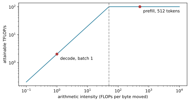
Raw FLOPs, however, do not predict speed, because a processor can starve for data. The roofline model(Williams et al. 2009) makes this one picture: plot attainable throughput against arithmetic intensity — FLOPs performed per byte moved from memory. Below the machine’s balance point (its peak FLOPs divided by its memory bandwidth), performance is capped by the bandwidth line, not the compute ceiling. Generating one token at batch 1 reads every weight to do just two FLOPs with each — intensity around 1 — while processing a long prompt reuses each loaded weight across every position in the prompt. The two phases of the same model sit on opposite sides of the roof:
Figure 2.3: Why is generating one token so much slower per FLOP than processing a prompt? On a machine with a 50 FLOP/byte balance point, single-token decode (intensity about 1) sits deep in the bandwidth-bound region at about 2% of peak, while a 512-token prefill reuses each loaded weight 512 times and reaches the compute ceiling.
Figure 2.3 is the single most economical explanation of inference behavior we will meet: prefill is compute-bound, decode is memory-bandwidth-bound, and no kernel wizardry moves a workload’s intensity — only batching, caching, and quantization do, which is Chapter 10’s subject matter. Keep the two dots in mind; they explain why time-to-first-token and time-per-output-token, measured in Section 1.6, obey different budgets.
2.8 Training: watch it learn
Everything is assembled; now we train it and watch. The optimizer is AdamW: Adam’s per-parameter step sizes from running moment estimates, with weight decay applied as a separate decoupled subtraction rather than mixed into the adaptive gradient — the difference that gives the W its name and makes decay behave like true regularization (Loshchilov and Hutter 2019). The learning rate follows the standard shape: a brief linear warmup (large steps under empty moment estimates are dangerous), then a smooth cosine decay to a small floor. And we clip the global gradient norm at 1.0, which bounds the damage of any single bad batch without pretending to fix its cause.
# @savedef lr_schedule(step: int, total_steps: int, peak: float) ->float:"""Return the learning rate for one step of warmup-then-cosine decay. The first 5% of steps ramp linearly from near zero to ``peak`` while optimizer moment estimates fill; the remainder follows a half cosine from ``peak`` down to one tenth of it. Args: step: The current optimizer step, from 0. total_steps: Total steps in the run. peak: The maximum learning rate. Returns: The learning rate to apply at this step. """ warmup =max(1, total_steps //20)if step < warmup:return peak * (step +1) / warmup progress = (step - warmup) /max(1, total_steps - warmup -1)return peak * (0.1+0.9*0.5* (1+ math.cos(math.pi * progress)))
A loss number on data the model is training on cannot tell us about generalization, so we hold out the final 15% of the token stream untouched and evaluate on it periodically:
split =int(0.85* data.numel())train_stream, val_stream = data[:split], data[split:]print(f"train: {train_stream.numel():,} tokens validation: {val_stream.numel():,} tokens")@torch.inference_mode()def heldout_loss(model: TinyGPT, tokens: torch.Tensor, windows: int=4) ->float:"""Average the loss over fixed windows of a stream the model never trains on.""" model.eval() block = model.config.block_size starts = torch.linspace(0, tokens.numel() - block -1, windows).long() losses = [ model(tokens[s : s + block][None], tokens[s +1 : s + block +1][None])[1].item()for s in starts ]returnsum(losses) /len(losses)
train: 3,325 tokens validation: 587 tokens
We also want to see what training changes inside the model, not just in its loss. The helper below recomputes one layer’s attention pattern for a prompt, and we snapshot it now, before any training, for comparison afterwards.
# @save@torch.inference_mode()def attention_weights(model: TinyGPT, token_ids: list[int], layer: int=0) -> Tensor:"""Recompute one layer's per-head attention pattern for a prompt. Runs the embedding and the blocks below ``layer`` to reproduce that layer's input, then reapplies its QKV projections and causal softmax. Each returned row is a probability distribution over visible positions. Args: model: A ``TinyGPT`` whose pattern we want to inspect. token_ids: The prompt as a list of token IDs. layer: Which block's attention to extract, from 0. Returns: Weights shaped ``(n_heads, T, T)``; rows sum to 1 and the upper triangle is exactly zero. """ model.eval() tokens = torch.tensor([token_ids]) positions = torch.arange(tokens.size(1)) x = model.token_embedding(tokens) + model.position_embedding(positions)for block in model.blocks[:layer]: x, _ = block(x) attn = model.blocks[layer].attention normed = model.blocks[layer].attention_norm(x) batch, steps, _ = normed.shape qkv = attn.qkv(normed).view(batch, steps, 3, attn.n_heads, attn.head_dim) query, key, _ = qkv.permute(2, 0, 3, 1, 4).unbind(0) query, key = attn.q_norm(query), attn.k_norm(key) scores = query @ key.transpose(-2, -1) / math.sqrt(attn.head_dim) mask = torch.triu(torch.ones(steps, steps, dtype=torch.bool), diagonal=1)return scores.masked_fill(mask, float("-inf")).softmax(dim=-1)[0]
probe_ids = tokenizer.encode("The rabbit-hole went straight on like a tunnel")weights_before = attention_weights(model, probe_ids)print("pattern shape:", tuple(weights_before.shape), " rows sum to", weights_before.sum(-1).mean().item())
pattern shape: (4, 19, 19) rows sum to 1.0
Now the loop itself — deliberately plain PyTorch, because this exact sequence of calls (batch, schedule, zero, forward, backward, clip, step) reappears in every training chapter of this book. We record the training loss at every step, the held-out loss every 25, and freeze a generated sample at two checkpoints so we can watch the model’s voice change.
400 steps in 23.4s (17 steps/s)
train loss: 6.261 -> 0.136 (mean of last 10)
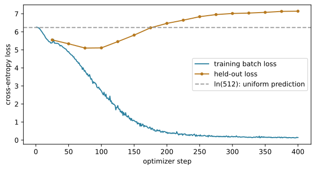
held-out loss: minimum 5.100 at step 75, then up to 7.143 at step 400
The train loss has collapsed; the held-out loss has not. Figure 2.4 shows both curves against the \ln V baseline, and it is the most instructive figure in the chapter precisely because it is not a success story.
Figure 2.4: What does this training run actually demonstrate? Training loss falls from the ln(512) uniform baseline toward zero, but held-out loss bottoms out inside the first hundred steps and then climbs: a 140K-parameter model is memorizing a 3.9K-token corpus, not learning English.
Read Figure 2.4 the way an engineer reads any loss curve — as a set of questions. The first point checks initialization: training loss starts at the uniform baseline, so no label is leaking (a start far below\ln V is the signature of the missing-mask bug from Section 2.4). The early descent shows the whole gradient path works. Then the curves split: training loss keeps falling toward zero while held-out loss bottoms out before step 100 and turns upward. That divergence is overfitting in its purest form — our model has roughly 42 parameters per training token, so it can simply memorize the stream, and does. At pretraining scale the ratio is reversed by orders of magnitude (Chapter 5), which is why frontier base-model curves show the two losses moving together. The same diagnostic stance handles the other shapes you will meet: a flat curve at \ln V means gradients are not reaching parameters; a spike mid-run means data, precision, or learning rate changed; a smooth curve with terrible samples means the objective and the hope were never aligned.
The samples tell the same story in prose. Here is the model at step 100 and at step 400, and the untrained byte soup from Section 2.6 for comparison:
step 100: 'Alice had usI sme ind in her Dinaaheds s isten see whe’t hed all ry th the s'
step 400: 'Alice think it so _ the Dinah; t much out of the cover.\n\nAlice think it so _very'
The step-100 sample is this book’s version of d2l’s famous 'it has in the the the': word-shaped fragments with real spacing — in her, see, th the s — and no meaning anywhere. The model has learned the texture of English (which merges tend to follow which) but none of its structure. By step 400 the output reads like Carroll, and that is exactly the problem: it reads like Carroll because it largely is Carroll — think it so _very_ much out of the is a span of the training text, complete with Gutenberg’s underscore italics, spliced awkwardly onto “Alice”. Greedy decoding makes the memorization plainest:
greedy: 'Alice think it so _very_ much out of the way to hear the Rabbit say to itself, “Oh dear! Oh dear! I shall '
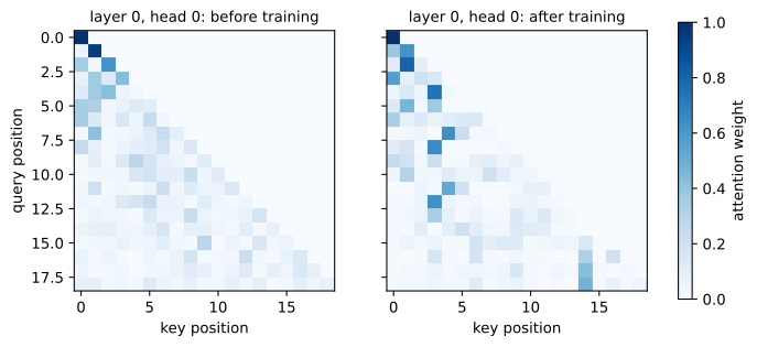
An honest summary of the artifact: mechanism demonstrated, competence absent. Everything a real pretraining run adds — a corpus millions of times larger than the model, deduplication, an actual data pipeline — exists to keep that held-out curve falling, and is the subject of Chapter 5. Meanwhile, training visibly reorganized the model’s internals. Figure 2.5 compares the layer-0 attention pattern we snapshotted before training with the same pattern now.
Figure 2.5: What did training do to attention? Before training (left), a layer-0 head spreads its weight broadly over the visible prefix; after training (right), the same head commits — many rows place half or more of their mass on one informative earlier token (the ‘abb’ of ‘rabbit’ collects much of it) instead of averaging everything.
Both panels are strictly lower-triangular — the mask holds no matter what the weights learn — but the texture changes from indiscriminate averaging to committed lookups. This is what “training the attention” means, one head at a time.
2.9 Generation and the KV cache
Look back at the generation loop in generate: without caching, producing token t+1 feeds all t existing tokens through every layer again. But their keys and values cannot have changed — the causal mask guarantees that earlier positions never see later ones, so their projections are frozen the moment they are computed. Recomputing them is pure waste. The KV cache stores, per layer, the keys and values of every position seen so far; each new step then projects only the newest token, appends its key and value, and attends its single query over the whole cache. That is precisely what CausalSelfAttention does when past is not None, and the absolute-position masking we wrote there makes the cached path compute the same function as the full one.
“The same function” is a testable claim, not a slogan. We generate greedily both ways and compare, then push a single token through the cached path against a full recomputation and measure the worst logit disagreement:
The tokens match exactly and the logits agree to within float32 roundoff (the two paths batch their matrix products differently, so bit-identity is not owed — functional identity is). Now the accounting, where a popular claim needs careful surgery. Per decoded token, the cache reduces projection work from O(t) recomputed positions to O(1) — one new token through the weights, regardless of prefix length. But the attention step itself still scores the new query against all t cached keys and mixes t values: O(t) compute per step, and the cache occupies O(t) memory. For multi-head attention the storage is exact and predictable:
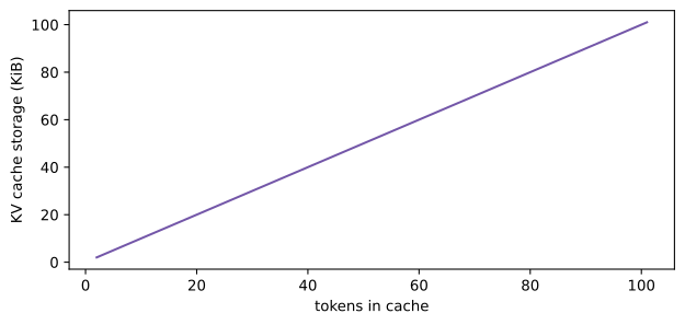
\text{cache bytes} = 2\,B\,L\,T\,d\,s,
\tag{2.6}
with batch B, L layers, T cached positions, model width d (keys and values each store H\,d_h=d scalars per layer per position — hence the 2), and s bytes per scalar. Both claims are checkable on our toy, so we check them. We extend a prefix 100 times; at each length we time a cached step and a full recomputation (taking the best of five runs each, the standard defense against timer noise at millisecond scale) and read the cache’s true storage from its tensors:
# @savedef kv_cache_bytes(cache: list[LayerCache]) ->int:"""Return the storage bytes occupied by all cached keys and values."""returnsum(t.numel() * t.element_size() for pair in cache for t in pair)
def best_of(runs: int, call) ->float:"""Return the fastest of several timed calls, in milliseconds.""" times = []for _ inrange(runs): tick = time.perf_counter() call() times.append((time.perf_counter() - tick) *1000)returnmin(times)model.eval()context = prompt.clone()cached_ms, full_ms, cache_sizes, prefix_lengths = [], [], [], []with torch.inference_mode(): logits, _, cache = model(context)for _ inrange(100): next_token = logits[:, -1].argmax(dim=-1, keepdim=True) context = torch.cat((context, next_token), dim=1) cached_ms.append(best_of(5, lambda: model(next_token, cache=cache))) full_ms.append(best_of(5, lambda: model(context))) logits, _, cache = model(next_token, cache=cache) prefix_lengths.append(context.size(1)) cache_sizes.append(kv_cache_bytes(cache))print(f"cached step: {cached_ms[0]:.2f} ms at prefix {prefix_lengths[0]}, "f"{cached_ms[-1]:.2f} ms at prefix {prefix_lengths[-1]}")print(f"full forward: {full_ms[0]:.2f} ms at prefix {prefix_lengths[0]}, "f"{full_ms[-1]:.2f} ms at prefix {prefix_lengths[-1]}")
cached step:   0.63 ms at prefix 2, 0.62 ms at prefix 101
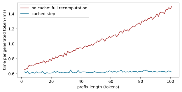
full forward:  0.65 ms at prefix 2, 1.50 ms at prefix 101
Figure 2.6: What work does the cache actually avoid? The full-recomputation cost climbs steadily with prefix length — every step re-pays for the entire past — while the cached step stays flat: constant projection work, plus an O(t) attention term too small to register at this width.
The uncached cost more than doubles across a hundred tokens of prefix — every step re-pays for the whole past — while the cached line is flat to within measurement noise. That flatness deserves an honest caveat rather than a cheer: the cached step’s O(t) attention term is present in the code, but at d=64 it amounts to a few tens of thousands of FLOPs — microseconds, invisible next to the fixed projection cost. At production scale, with tens of thousands of cached positions across dozens of layers, that same term and the cache’s memory footprint come to dominate the step — which is why “KV caching makes decoding O(1)” is a claim to correct, not repeat. Storage tells its side of the story with perfect predictability:
fig, ax = plt.subplots(figsize=(6.6, 3.2))ax.plot(prefix_lengths, [size /1024for size in cache_sizes], color="#7356a8")ax.set_xlabel("tokens in cache")ax.set_ylabel("KV cache storage (KiB)")fig.tight_layout()plt.show()
Figure 2.7: Does cache storage follow the formula? Measured bytes climb by exactly 2BLds = 1,024 bytes per cached token — memory per generation step is O(n) even though projection compute is O(1).
Every cached token costs 1,024 bytes here — Equation 2.6 with our constants, verified against the tensors themselves. Substitute a production configuration into the same formula and the number stops being cute; Chapter 3 does that arithmetic and then spends most of its pages on the architectural responses (grouped and compressed KV heads, sliding windows) that exist to shrink it. Finally, the end-to-end payoff at our scale:
for use_cache in (True, False): tick = time.perf_counter() generate(model, torch.tensor([tokenizer.encode("Alice was ")]), 110, use_cache=use_cache) seconds = time.perf_counter() - tickprint(f"use_cache={str(use_cache):5s}: {110/ seconds:6.0f} tokens/s")
A solid speedup from a dictionary of tensors and zero change in output — and the gap widens with every token of prefix, every layer, and every unit of width. This measurement, more than any diagram, is why every serving stack in Chapter 10 is organized around keeping, sharing, and paging these caches.
NoteIn the interview
Q. A teammate says “the KV cache makes generation O(1) per token.” Where is that right, and where is it wrong? Right for projection work: each step pushes one token, not t, through the weights. Wrong for the attention step (the new query still scores and mixes t cached entries — O(t) compute) and wrong for memory ({2BLTds} bytes, growing linearly). The trap is accepting the claim whole; the strong answer splits it into the three terms and names the measurement — per-step latency and cache bytes versus prefix length — that would show each one.
2.10 Summary
We built a GPT from its parts and watched every claim execute: a byte-level BPE tokenizer with zero unknown tokens and a frozen 512-entry vocabulary; attention derived as a scaled softmax lookup, with the \sqrt{d_k} earned from a measured variance blowup; a causal mask verified bit-for-bit; blocks that add updates to a residual stream; a tied head whose savings we counted. Training collapsed the train loss while the held-out loss rose — memorization, honestly diagnosed — and cached generation reproduced uncached logits while its storage grew by exactly {2BLds} bytes per token. Chapter 3 now asks what happens when the context, and that cache, get long.
2.11 Exercises
Expose the cheat. Delete the masked_fill line from CausalSelfAttention.forward and rerun the training loop. (a) Predict where the training loss will start and where it will go, then check. (b) Rerun the future-change probe from Section 2.4 and report the earlier-position drift. (c) Explain why the held-out loss also improves — and why that makes the bug more dangerous, not less.
Trade heads for width. Double n_heads to 8 while holding d_model at 64. Use param_breakdown and Equation 2.6 to predict which parameter and cache terms change before you run anything, then verify with parameter_count and kv_cache_bytes. What did change, given that the totals did not?
Audit the tokenizer’s domain. Train a second 512-entry BytePairTokenizer on a few kilobytes of Python source instead of Carroll. Compare the first 16 merges, then measure bytes-per-token for each tokenizer on the other corpus. Where does the fertility penalty come from, and at what point in a model’s life is it locked in?
Untie the head. Remove the weight-tying line from TinyGPT.__init__, predict the new parameter count with param_breakdown plus Vd, verify it, and train for 400 steps at three seeds. Does the extra capacity buy anything measurable on the held-out stream at this scale?
Slow the memorization. Using the loss curve in Figure 2.4 as the baseline, find the combination of weight_decay, model width, and step count that yields the lowest held-out loss you can reach on this corpus. Report the best curve and where its minimum sits relative to step 100.
Account for a real model. A 7B-class configuration is roughly V=32{,}000, d=4{,}096, h=11{,}008, L=32, H=32. Run param_breakdown and flops_per_token on it, report which components dominate compared with our toy, and compute its KV cache bytes per token at fp16 from Equation 2.6. State explicitly what the estimate omits.
Place decode on the roofline. Using Figure 2.3’s machine (100 TFLOP/s, 2 TB/s), estimate the arithmetic intensity of batch-8 decode and of a 128-token prefill for the 7B configuration from Exercise 6, place both on the roofline, and state which knob a serving team turns to move each point — then check your reasoning against Chapter 10’s batching sections.
Loshchilov, Ilya, and Frank Hutter. 2019. “Decoupled Weight Decay Regularization.”International Conference on Learning Representations.
Press, Ofir, and Lior Wolf. 2017. “Using the Output Embedding to Improve Language Models.”Proceedings of the Conference of the European Chapter of the Association for Computational Linguistics.
Radford, Alec, Jeffrey Wu, Rewon Child, David Luan, Dario Amodei, and Ilya Sutskever. 2019. “Language Models Are Unsupervised Multitask Learners.”OpenAI Technical Report.
Sennrich, Rico, Barry Haddow, and Alexandra Birch. 2016. “Neural Machine Translation of Rare Words with Subword Units.”Proceedings of the Annual Meeting of the Association for Computational Linguistics.
Vaswani, Ashish et al. 2017. “Attention Is All You Need.”Advances in Neural Information Processing Systems.
Williams, Samuel, Andrew Waterman, and David Patterson. 2009. “Roofline: An Insightful Visual Performance Model for Multicore Architectures.”Communications of the ACM.
Zhang, Biao, and Rico Sennrich. 2019. “Root Mean Square Layer Normalization.”Advances in Neural Information Processing Systems.