# @save
from dataclasses import dataclass


@dataclass(frozen=True)
class KVConfig:
    """Architectural quantities that fix a model's persistent KV state.

    These are exactly the fields @eq-ch03-kvbytes multiplies together. A
    standard attention layer stores ``2 * kv_heads * head_dim`` scalars per
    layer per token; a latent (MLA) layer overrides that with a compressed
    width, which is why the stored width is a method rather than a constant.

    Args:
        name: A label used in tables and plots.
        layers: Number of attention layers, ``L``.
        query_heads: Number of query heads, ``H_q`` (state-neutral; kept for
            the MHA/GQA ratio).
        head_dim: Dimensions per cached head, ``d_h``.
        bytes_per_scalar: Cache dtype width ``s`` (2 for fp16/bf16, 1 for int8).
        kv_heads: Key-value heads ``H_kv`` for standard attention; ``None`` for
            a latent cache.
        latent_rank: Width ``r`` of an MLA latent, when the cache is compressed.
        rope_key_dim: Width ``d_R`` of an MLA decoupled rotary key, cached
            alongside the latent.
    """

    name: str
    layers: int
    query_heads: int
    head_dim: int
    bytes_per_scalar: int
    kv_heads: int | None = None
    latent_rank: int | None = None
    rope_key_dim: int = 0

    def cached_scalars_per_layer_token(self) -> int:
        """Return the stored scalar width per layer per token.

        Standard attention stores ``2 * H_kv * d_h`` (keys and values); a
        latent cache stores ``r + d_R`` (the compressed latent plus its
        decoupled rotary key). This is the only place the two cache designs
        differ in the byte accounting.
        """
        if self.latent_rank is not None:
            return self.latent_rank + self.rope_key_dim
        if self.kv_heads is None:
            raise ValueError("standard attention requires kv_heads")
        return 2 * self.kv_heads * self.head_dim


def kv_bytes(config: KVConfig, tokens: int, batch: int = 1) -> int:
    """Return payload bytes for one append-only, unquantized KV cache.

    This is the book's canonical KV-byte declaration (@eq-ch03-kvbytes). It is
    tensor payload only: it excludes allocator metadata, padding, temporary
    attention workspaces, and tensor-parallel duplication, all of which a
    deployment capacity model (Chapter 10) adds on top.

    Args:
        config: The architecture whose cache we are sizing.
        tokens: Retained tokens per sequence, ``T``.
        batch: Sequences represented at once, ``B``.

    Returns:
        Total cache payload in bytes.

    Raises:
        ValueError: If ``tokens`` is negative or ``batch`` is not positive.
    """
    if tokens < 0 or batch < 1:
        raise ValueError("tokens must be nonnegative and batch positive")
return batch * tokens * config.layers * config.cached_scalars_per_layer_token() * config.bytes_per_scalar3 Attention, Position, and Long Context
In Chapter 2 we gave TinyGPT a learned absolute position table and called it a placeholder (Section 2.6), and we watched its KV cache grow at exactly {2BLds} bytes per token (Section 2.9). This chapter cashes in both. The position table is replaced by rotary embeddings, which encode relative offset and can be stretched to longer contexts. And that innocuous {2BLds}, evaluated at a production scale, becomes the central cost of long context.
Here is the shock in one number. An agent has spent an hour reading a repository, opening issues, running tests, and refining a patch; its transcript reaches 128K tokens. The next request adds four words — “now fix the race.” For a conventional 32-layer, 32-head model with 128-dimensional heads and two-byte cached scalars, that one conversation’s keys and values occupy 64 GiB — payload alone, before weights, activations, or allocator slack. At 4K tokens the same state is 2 GiB. Context grew by 32×; persistent attention state grew by 32× with it.
We build the mechanisms that bend that curve, in small executed pieces: (i) a KV-byte calculator we run against real model configs; (ii) grouped-query and latent attention layers whose caches we shrink and measure; (iii) sliding-window and attention-sink masks we visualize and price; (iv) RoPE derived from rotation, with its relative-offset invariant printed live; (v) the PI, NTK, and YaRN recipes that reshape RoPE’s frequency bands; and (vi) a synthetic retrieval-versus-position probe — the chapter’s flagship figure — measured before and after scaling. Three questions organize the work: capacity (how many bytes stay live?), computation (how much work per token?), and capability (does the model actually use the evidence?).
3.1 The KV-cache equation
Start from one layer. During autoregressive decoding the query projections are transient, but every retained token contributes one key and one value per KV head that must persist so the next token can attend over the whole history. Multiply that per-token slice out over the model and we have the whole cost. Define:
| Symbol | Meaning |
|---|---|
| B | sequences represented in the cache |
| T | retained tokens per sequence |
| L | attention layers |
| H_{kv} | key-value heads per layer |
| d_h | dimensions in each cached head |
| s | bytes per cached scalar |
The payload is
\operatorname{KVBytes}=B\,T\,L\,(2\,H_{kv}\,d_h)\,s. \tag{3.1}
The factor of two is not a safety margin — it is one tensor for keys and one for values. H_{kv}d_h is the width of each tensor’s per-token slice; multiplying by layers, tokens, batch, and scalar width counts every stored element. Equation 3.1 assumes a uniform architecture, equal key and value widths, and an append-only, unquantized cache. We write it once, as the book’s canonical KV function, with a small config object so an unusual cache can declare its own stored width without a second formula.
The opening 64 GiB now follows from the function, not from arithmetic in the margin. We instantiate the 32-layer MHA model and read off the per-token slice and the two headline totals.
mha = KVConfig("MHA 7B-class", layers=32, query_heads=32, kv_heads=32, head_dim=128, bytes_per_scalar=2)
per_token = kv_bytes(mha, 1)
print(f"per token: {per_token:,} bytes = {per_token / 1024:.0f} KiB")
print(f"at   4,096 tokens: {kv_bytes(mha,   4_096) / 2**30:.2f} GiB")
print(f"at 131,072 tokens: {kv_bytes(mha, 131_072) / 2**30:.2f} GiB")
per token: 524,288 bytes = 512 KiB
at 4,096 tokens: 2.00 GiB
at 131,072 tokens: 64.00 GiBHalf a mebibyte per token, and the totals are exact: 2 GiB at 4K, 64 GiB at 128K. Before we spend the chapter shrinking that number, one complexity myth needs correcting, because it hides the computation question behind the capacity one. In Chapter 2 we measured the cache reproducing uncached logits while its storage grew linearly (Section 2.9). What the cache avoids is reprojecting old tokens — O(1) projection work per step instead of O(T). It does not avoid reading those keys and values: the new query still scores against all T of them and mixes T values, so decode attention stays O(T) per step and memory stays O(T). “The KV cache makes generation O(1)” confuses avoided projection with total work.
Real models fight the byte count with architecture, and the differences are visible the moment we plug their published configs into the same function. Multi-query and grouped-query models cut H_{kv}; latent models replace {2H_{kv}d_h} with a compressed width. We build three configs from dated public sources and sweep them over context length.
# Fields taken from published config.json files (see the Verify-live box below).
llama2 = KVConfig("Llama 2 7B (MHA)", layers=32, query_heads=32, kv_heads=32, head_dim=128, bytes_per_scalar=2)
llama31 = KVConfig("Llama 3.1 8B (GQA-8)", layers=32, query_heads=32, kv_heads=8, head_dim=128, bytes_per_scalar=2)
deepseek = KVConfig("DeepSeek-V2-Lite (MLA)", layers=27, query_heads=16, head_dim=128,
                    bytes_per_scalar=2, latent_rank=512, rope_key_dim=64)

contexts = (4_096, 16_384, 32_768, 65_536, 131_072)
print(f"{'context':>9} | {'Llama 2 MHA':>12} | {'Llama 3.1 GQA':>13} | {'DeepSeek MLA':>12}")
for t in contexts:
    row = [kv_bytes(cfg, t) / 2**30 for cfg in (llama2, llama31, deepseek)]
    print(f"{t:>9,} | {row[0]:>9.2f} GiB | {row[1]:>10.2f} GiB | {row[2]:>9.3f} GiB")
context | Llama 2 MHA | Llama 3.1 GQA | DeepSeek MLA
4,096 | 2.00 GiB | 0.50 GiB | 0.119 GiB
16,384 | 8.00 GiB | 2.00 GiB | 0.475 GiB
32,768 | 16.00 GiB | 4.00 GiB | 0.949 GiB
65,536 | 32.00 GiB | 8.00 GiB | 1.898 GiB
131,072 | 64.00 GiB | 16.00 GiB | 3.797 GiBRead the 64K row: a single Llama 3.1 8B conversation at 64K tokens holds 8 GiB of KV cache — 8.6 GB in the decimal units a datasheet quotes — and eight such sessions fill an 80 GB accelerator before any weights load. The GQA column is exactly one quarter of the MHA column (8 KV heads instead of 32), and the MLA column is smaller again. Figure 3.1 plots the three slopes.
Show the code that draws this figure
import matplotlib.pyplot as plt

fig, ax = plt.subplots(figsize=(6.6, 3.7))
styles = [("#b13f3f", "s", "--"), ("#2a7f9e", "^", "-"), ("#7356a8", "o", ":")]
for cfg, (color, marker, ls) in zip((llama2, llama31, deepseek), styles):
    xs = [t / 1024 for t in contexts]
    ys = [kv_bytes(cfg, t) / 2**30 for t in contexts]
    ax.plot(xs, ys, marker=marker, linestyle=ls, color=color, label=cfg.name)
ax.set_xlabel("context represented in cache (Ki tokens)")
ax.set_ylabel("KV payload (GiB)")
ax.legend()
fig.tight_layout()
plt.show()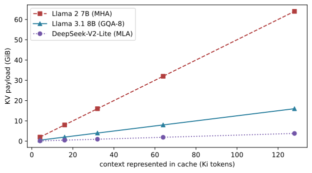
NoteLandscape 2026 — the config numbers behind the plot
The three configs are read from published files: Llama 2 7B (32 heads, MHA), Llama 3.1 8B (num_key_value_heads: 8, GQA), and DeepSeek-V2-Lite (kv_lora_rank: 512, qk_rope_head_dim: 64, MLA). They pin cache accounting fields only; real allocated memory is higher and differently sharded.
Verify live: re-download each config.json, map num_key_value_heads, head_dim, num_hidden_layers, and torch_dtype onto KVConfig, and recompute before using a row in a capacity decision. Verified: 2026-07-19.
3.2 Share keys and values: MQA and GQA
Multi-head attention gives every query head its own key and value head. But the query projections vanish after each step; only the keys and values persist. So the cheapest lever on cache size is to let several query heads share one key-value head. If H_q=H_{kv} we have ordinary multi-head attention (MHA). Collapse all query heads onto a single KV head (H_{kv}=1) and we have multi-query attention (MQA) (Shazeer 2019). Anything in between is grouped-query attention (GQA) (Ainslie et al. 2023): with H_q=32 and H_{kv}=8, each KV head serves a group of four query heads, which keep their own queries and so can still ask different questions.
The cache ratio against MHA falls straight out of Equation 3.1, since only H_{kv} changes:
\frac{\operatorname{KVBytes}_{\text{grouped}}}{\operatorname{KVBytes}_{\text{MHA}}}=\frac{H_{kv}}{H_q}. \tag{3.2}
This counts stored elements, not quality — the GQA paper showed an MHA checkpoint can be converted by grouping heads and briefly uptrained, recovering most of the quality at close to MQA speed. We build one layer whose kv_heads dial spans all three regimes, cache the compact keys and values, and expand groups only for the score computation.
# @save
import torch
from torch import Tensor, nn
from torch.nn import functional as F


class GroupedQueryAttention(nn.Module):
    """Causal attention whose kv-head dial spans MHA, GQA, and MQA.

    Queries get ``query_heads`` full heads; keys and values get only
    ``kv_heads`` heads, which is all that is cached. At read time each KV head
    is repeated to serve its group of query heads, so the stored state shrinks
    by ``kv_heads / query_heads`` while the output shape is unchanged. A
    production kernel repeats the heads implicitly; we materialize them so the
    mechanism is visible.
    """

    def __init__(self, d_model: int, query_heads: int, kv_heads: int) -> None:
        super().__init__()
        if d_model % query_heads or query_heads % kv_heads:
            raise ValueError("query_heads must divide width and be divisible by kv_heads")
        self.query_heads, self.kv_heads = query_heads, kv_heads
        self.head_dim = d_model // query_heads
        self.q_proj = nn.Linear(d_model, query_heads * self.head_dim, bias=False)
        self.k_proj = nn.Linear(d_model, kv_heads * self.head_dim, bias=False)
        self.v_proj = nn.Linear(d_model, kv_heads * self.head_dim, bias=False)
        self.out_proj = nn.Linear(d_model, d_model, bias=False)

    def forward(self, x: Tensor, cache: tuple[Tensor, Tensor] | None = None) -> tuple[Tensor, tuple[Tensor, Tensor]]:
        """Run causal attention and return the output and the compact KV cache.

        The returned cache holds only ``kv_heads`` heads; group expansion
        happens after it, so what is stored follows ``kv_heads`` while the
        computation still uses ``query_heads``.
        """
        batch, query_len, _ = x.shape
        q = self.q_proj(x).view(batch, query_len, self.query_heads, self.head_dim).transpose(1, 2)
        k = self.k_proj(x).view(batch, query_len, self.kv_heads, self.head_dim).transpose(1, 2)
        v = self.v_proj(x).view(batch, query_len, self.kv_heads, self.head_dim).transpose(1, 2)
        if cache is not None:
            k = torch.cat((cache[0], k), dim=2)
            v = torch.cat((cache[1], v), dim=2)
        present = (k, v)  # compact: only kv_heads heads are stored
        repeats = self.query_heads // self.kv_heads
        scores = q @ k.repeat_interleave(repeats, dim=1).transpose(-2, -1) / self.head_dim**0.5
        past = k.size(2) - query_len
        q_pos = past + torch.arange(query_len)[:, None]
        k_pos = torch.arange(k.size(2))[None, :]
        weights = F.softmax(scores.masked_fill(k_pos > q_pos, float("-inf")), dim=-1)
        out = (weights @ v.repeat_interleave(repeats, dim=1)).transpose(1, 2).reshape(batch, query_len, -1)
        return self.out_proj(out), present
We turn the dial across the four heads → one head range and read the cache each setting stores. The output shape must never move; only the cached tensor’s head axis does.
torch.manual_seed(3)
x = torch.randn(1, 8, 64)                     # width 64, 8 query heads -> head_dim 8
for kv_heads, tag in [(8, "MHA"), (2, "GQA-2"), (1, "MQA")]:
    layer = GroupedQueryAttention(64, query_heads=8, kv_heads=kv_heads)
    out, (k, v) = layer(x)
    scalars = k.numel() + v.numel()
    print(f"{tag:6s} kv_heads={kv_heads}: cache {tuple(k.shape)} x2  "
          f"= {scalars:4d} scalars   out {tuple(out.shape)}   ratio {kv_heads/8:.3f}")
MHA kv_heads=8: cache (1, 8, 8, 8) x2 = 1024 scalars out (1, 8, 64) ratio 1.000
GQA-2 kv_heads=2: cache (1, 2, 8, 8) x2 = 256 scalars out (1, 8, 64) ratio 0.250
MQA kv_heads=1: cache (1, 1, 8, 8) x2 = 128 scalars out (1, 8, 64) ratio 0.125The output stays [1,8,64] throughout while the cache drops from 1024 scalars (MHA) to 128 (MQA) — exactly the {1/8} ratio Equation 3.2 predicts. Shrinking the cache is only legal if the cheaper path still computes the same function, so we prove it: feed the sequence one token at a time through the cache and check the incremental outputs against a single full pass.
layer = GroupedQueryAttention(64, query_heads=8, kv_heads=2).eval()
full, _ = layer(x)
cache, pieces = None, []
for t in range(x.size(1)):
    step, cache = layer(x[:, t:t+1], cache)
    pieces.append(step)
incremental = torch.cat(pieces, dim=1)
print("cached == full:", torch.allclose(incremental, full, atol=1e-6),
      f"  max gap {(incremental - full).abs().max().item():.1e}")
cached == full: True max gap 1.8e-07The grouped cache reproduces the full-attention output to float roundoff. Figure 3.2 draws what “grouped” means physically: query heads fan into a shrinking set of shared KV heads.
flowchart TB
    subgraph MHA["MHA (8 KV heads, ratio 1)"]
      direction TB
      q0["q0..q7"] --> k0["8 KV heads"]
    end
    subgraph GQA["GQA-2 (2 KV heads, ratio 1/4)"]
      direction TB
      g0["q0..q3"] --> kg0["KV head A"]
      g1["q4..q7"] --> kg1["KV head B"]
    end
    subgraph MQA["MQA (1 KV head, ratio 1/8)"]
      direction TB
      m0["q0..q7"] --> km0["1 KV head"]
    end
One caveat carries into Chapter 10: our layer materializes the repeated heads, but a serving kernel must expand them implicitly, or the byte saving is spent again on memory traffic. Kernel support gates whether an architectural win survives on real hardware.
3.3 Compress the cache: MLA
Sharing heads picks fewer full-width key-value representations. A different lever keeps all the heads but stores them compressed. Multi-head latent attention (MLA), introduced with DeepSeek-V2 (DeepSeek-AI 2024), projects the residual state down to a small latent from which the per-head keys and values are reconstructed on read.
For residual state x_t\in\mathbb{R}^{d}, a down-projection forms the cached latent, and per-head up-projections reconstruct content keys and values:
c_t = W^{\!D}\,x_t,\qquad c_t\in\mathbb{R}^{r},\quad r\ll 2H_qd_h . \tag{3.3}
Only c_t is cached. There is a subtlety, though, that decides the whole design: RoPE (the next sections’ rotation) sits between the up-projection and the dot product, and it does not commute with W^{\!D}, so a purely latent key cannot also carry rotary position. DeepSeek’s fix is decoupled RoPE — a form of partial RoPE. The content key comes from the latent and carries no rotation; a small, separate rotary key of width d_R is projected, rotated, and cached alongside the latent. The score for query head i is a sum of a content term and a shared rotary term, and the stored width becomes r+d_R rather than {2H_{kv}d_h} — exactly the width the calculator used for DeepSeek’s 512 + 64 above. Figure 3.3 locates the two cached tensors.
flowchart LR
    X["residual x_t"] --> D["down-proj W_D"]
    D --> C["latent c_t  (CACHED)"]
    X --> R["rotary-key proj"]
    R --> KR["decoupled rope key  (CACHED)"]
    C --> UK["up-proj -> per-head K  (recomputed)"]
    C --> UV["up-proj -> per-head V  (recomputed)"]
We build the down/up latent path as an inspectable toy — deliberately not absorbing the projections the way a production kernel would, so the compress-reconstruct boundary stays on the page. The decoupled rotary band is what Figure 3.3 adds on top; here we measure the compression the latent buys.
# @save
class ToyLatentKVAttention(nn.Module):
    """Didactic MLA-style attention that caches one low-rank latent per token.

    The layer down-projects the residual to a rank-``latent_rank`` latent, caches
    only that, and up-projects it back to per-head keys and values at read time.
    Production MLA also absorbs the up-projections into the query and output
    maps so the per-head tensors are never materialized, and adds a decoupled
    rotary key of width ``rope_key_dim`` (@fig-ch03-mla-flow); we leave the
    boundary explicit and measure the latent compression on its own.
    """

    def __init__(self, d_model: int, query_heads: int, latent_rank: int, rope_key_dim: int = 0) -> None:
        super().__init__()
        if d_model % query_heads:
            raise ValueError("query_heads must divide d_model")
        self.query_heads = query_heads
        self.head_dim = d_model // query_heads
        self.latent_rank, self.rope_key_dim = latent_rank, rope_key_dim
        self.kv_down = nn.Linear(d_model, latent_rank, bias=False)
        self.k_up = nn.Linear(latent_rank, d_model, bias=False)
        self.v_up = nn.Linear(latent_rank, d_model, bias=False)
        self.q_proj = nn.Linear(d_model, d_model, bias=False)
        self.out_proj = nn.Linear(d_model, d_model, bias=False)

    def forward(self, x: Tensor, cache: Tensor | None = None) -> tuple[Tensor, Tensor]:
        """Run causal attention, caching (and returning) only the latent."""
        batch, query_len, _ = x.shape
        latent = self.kv_down(x)
        if cache is not None:
            latent = torch.cat((cache, latent), dim=1)
        key_len = latent.size(1)
        q = self.q_proj(x).view(batch, query_len, self.query_heads, self.head_dim).transpose(1, 2)
        k = self.k_up(latent).view(batch, key_len, self.query_heads, self.head_dim).transpose(1, 2)
        v = self.v_up(latent).view(batch, key_len, self.query_heads, self.head_dim).transpose(1, 2)
        scores = q @ k.transpose(-2, -1) / self.head_dim**0.5
        q_pos = (key_len - query_len) + torch.arange(query_len)[:, None]
        k_pos = torch.arange(key_len)[None, :]
        weights = F.softmax(scores.masked_fill(k_pos > q_pos, float("-inf")), dim=-1)
        out = (weights @ v).transpose(1, 2).reshape(batch, query_len, -1)
        return self.out_proj(out), latent

    def latent_width(self) -> int:
        """Return the stored width per token, ``r + d_R`` (@eq-ch03-kvbytes)."""
        return self.latent_rank + self.rope_key_dim
At width 64 with 4 heads, a standard cache stores {2H_qd_h}=128 scalars per token. We compress that to a rank-16 latent (plus a 4-wide decoupled rotary band for honest accounting) and measure both the ratio and that attention still works incrementally.
torch.manual_seed(11)
layer = ToyLatentKVAttention(64, query_heads=4, latent_rank=16, rope_key_dim=4).eval()
x = torch.randn(1, 8, 64)
full, latent = layer(x)

mha_width = 2 * 4 * (64 // 4)                  # 2 * H * d_h
stored = layer.latent_width()
print(f"standard cache: {mha_width} scalars/token   MLA latent: {stored} scalars/token"
      f"   ({mha_width / stored:.1f}x smaller)")

cache, pieces = None, []
for t in range(x.size(1)):
    step, cache = layer(x[:, t:t+1], cache)
    pieces.append(step)
print("cached == full:", torch.allclose(torch.cat(pieces, 1), full, atol=1e-6))
standard cache: 128 scalars/token MLA latent: 20 scalars/token (6.4x smaller)
cached == full: TrueA 6.4× smaller cache, and the incremental path still reproduces the full pass. The saving is real but not free: rank r bounds the information the latent can carry, the up- and down-projections cost parameters and compute, and — because production MLA absorbs those up-projections into the surrounding query and output maps so it never materializes per-head keys — the win depends on having a kernel that supports the absorbed path. Renaming projections does not compress an existing checkpoint; conversions such as TransMLA require deliberate uptraining.
3.4 Restrict visibility: windows, interleaving, and sinks
Sharing and compression keep full causal visibility — every query can still reach every past key. The third lever changes which keys a query may see at all. A sliding-window layer lets position t attend only to the most recent W positions. Its cached state per layer is bounded by substituting \min(T,W) for T in Equation 3.1, and its attention work per query is bounded by W. The price is architectural: anything older than W is unreachable through that layer.
The mask is the mechanism, so we build it directly — a boolean grid where cell (i,j) is true when query i may attend key j.
# @save
def visibility_mask(seq_len: int, window: int | None = None, sinks: int = 0) -> Tensor:
    """Return the boolean attention-visibility grid for one layer.

    Entry ``[i, j]`` is True when query position ``i`` may attend key position
    ``j``. With ``window=None`` this is the ordinary causal mask; a finite
    ``window`` keeps only the last ``W`` keys; ``sinks`` additionally keeps the
    first few positions always visible, the StreamingLLM pattern.

    Args:
        seq_len: Sequence length of the square grid.
        window: Sliding-window width ``W``; ``None`` for full causal.
        sinks: Number of initial "attention sink" positions kept visible.

    Returns:
        A ``(seq_len, seq_len)`` boolean tensor.
    """
    i = torch.arange(seq_len)[:, None]
    j = torch.arange(seq_len)[None, :]
    causal = j <= i
    if window is None:
        return causal
    return causal & (((i - j) < window) | (j < sinks))
We render three visibility patterns for a 12-token sequence: full causal, a width-4 window, and the same window with two sink positions pinned open. Figure 3.4 shows how much of the past each query can still reach.
Show the code that draws this figure
fig, axes = plt.subplots(1, 3, figsize=(8.4, 3.0))
panels = [("full causal", visibility_mask(12)),
          ("window W=4", visibility_mask(12, window=4)),
          ("window W=4 + 2 sinks", visibility_mask(12, window=4, sinks=2))]
for ax, (title, mask) in zip(axes, panels):
    ax.imshow(mask, cmap="Blues", vmin=0, vmax=1)
    ax.set_title(title, fontsize=10)
    ax.set_xlabel("key")
axes[0].set_ylabel("query")
fig.tight_layout()
plt.show()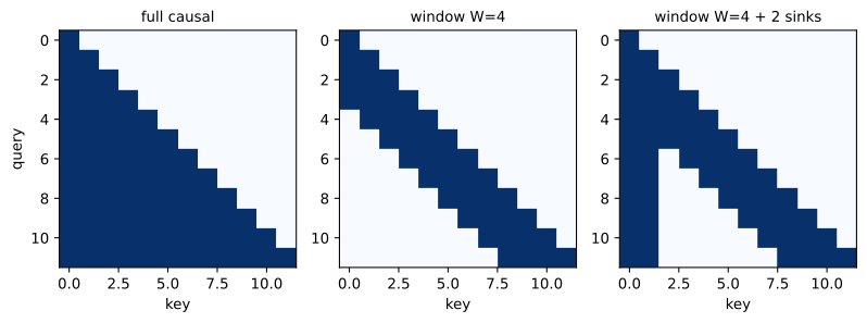
Stacking local layers widens the effective receptive field — an old token can influence a newer summary across layers — but indirect reach is not direct access, and exact copying or evidence attribution is sensitive to the difference. The common compromise interleaves local and full layers: local layers handle nearby structure cheaply, periodic global layers restore long-range paths. The total cache is then a sum, and it is worth computing rather than hand-waving. Take a 32-layer model at 128K tokens with a 4K window and every fourth layer global.
cfg = KVConfig("GQA-8", layers=32, query_heads=32, kv_heads=8, head_dim=128, bytes_per_scalar=2)
T, W = 131_072, 4_096
width_bytes = cfg.cached_scalars_per_layer_token() * cfg.bytes_per_scalar
global_layers, local_layers = 8, 24
full = kv_bytes(cfg, T)
interleaved = (global_layers * T + local_layers * min(T, W)) * width_bytes
print(f"all-global cache:   {full / 2**30:6.2f} GiB")
print(f"1:4 interleaved:    {interleaved / 2**30:6.2f} GiB   ({full / interleaved:.1f}x smaller)")
all-global cache: 16.00 GiB
1:4 interleaved: 4.38 GiB (3.7x smaller)Interleaving turns 16 GiB into under 3 GiB by keeping only a quarter of the layers full-range. But windows carry a failure mode discovered by StreamingLLM (Xiao et al. 2024): a naive rolling window that simply evicts old tokens can destabilize a trained model, even when the evicted tokens are semantically unimportant. The reason is that softmax must put its weight somewhere, and models learn to dump excess probability on the first few positions — attention sinks. Evict the sink and that mass has nowhere to go but the content tokens. We show the mechanism on a constructed score row where position 0 is the learned sink.
scores = torch.tensor([9.0, 1.0, 0.5, 1.2, 0.8, 1.1, 0.6, 1.3])   # pos 0 is the sink
full_attn = scores.softmax(0)
content = slice(4, 8)                         # the recent tokens a window keeps
naive = scores[content].softmax(0)            # rolling window: sink evicted, renormalize
sinked = scores[[0, 4, 5, 6, 7]].softmax(0)   # sink-aware window: keep position 0

def row(v):
    return f"{v.numpy().round(4)}  (sum {float(v.sum()):.4f})"

print(f"attention on tokens 4..7, full context:  {row(full_attn[content])}")
print(f"  naive window (sink evicted):           {row(naive)}")
print(f"  sink-aware window (position 0 kept):   {row(sinked[1:])}")
attention on tokens 4..7, full context: [0.0003 0.0004 0.0002 0.0005] (sum 0.0013)
naive window (sink evicted): [0.2076 0.2802 0.17 0.3422] (sum 1.0000)
sink-aware window (position 0 kept): [0.0003 0.0004 0.0002 0.0005] (sum 0.0013)With full context the four recent tokens together hold about a thousandth of the mass; the sink holds the rest. Drop the sink and that same query pours all of its attention onto those four tokens — their summed weight jumps from roughly 0.001 to 1.0, a change in the effective computation that is the instability StreamingLLM observed. Pin the sink open and the recent tokens keep their small, correctly-ordered weights (this is an illustration of the mechanism, not a measurement of a trained model). Sink retention is thus a masking-and-stability trick, not long-term memory: a visible sink token does not make an evicted tool result recoverable. Whether local, hybrid, or full attention wins is empirical — MiniMax’s M2 team reported choosing full attention in 2026 after hybrid variants degraded on long-context agent tasks, a useful counterexample to treating efficient patterns as free upgrades.
3.5 RoPE encodes relative position by rotation
Attention is permutation-blind: reorder the tokens and, before the causal mask, the outputs merely reorder with them. Chapter 2 patched that with a learned absolute position table. Let us look at what that placeholder actually is, using the model we built there.
import sys
sys.path.insert(0, "code/ch02")
import _generated as ch02                       # the model we built in Chapter 2

placeholder = ch02.TinyGPT(ch02.GPTConfig(vocab_size=512))
table = placeholder.position_embedding
print(f"learned absolute position table: {tuple(table.weight.shape)}")
print(f"positions it can represent: 0..{table.num_embeddings - 1}")
learned absolute position table: (128, 64)
positions it can represent: 0..127A fixed 128-row lookup: it cannot address position 128, and every row is learned independently, so nothing ties “50 and 51 are one apart” to “500 and 501 are one apart.” Rotary position embeddings (RoPE) replace it with something that encodes relative offset directly and extends past any trained length (Su et al. 2021). Take a coordinate pair (x_{2j},x_{2j+1}) and, at position m, rotate it by angle m\omega_j:
R_j(m)=\begin{bmatrix}\cos(m\omega_j)&-\sin(m\omega_j)\\ \sin(m\omega_j)&\cos(m\omega_j)\end{bmatrix},\qquad \omega_j=b^{-2j/d_R}. \tag{3.4}
Here d_R is the rotary width and b the frequency base. Small j gives a high-frequency band that spins fast; large j gives a low-frequency band that barely moves. RoPE rotates queries and keys (never values) by the block-diagonal collection of these rotations. Because rotation matrices are orthogonal they preserve norm, and — the point of the whole construction —
(R(m)q)^\top(R(n)k)=q^\top R(m)^\top R(n)k=q^\top R(n-m)k . \tag{3.5}
The score depends on m and n only through n-m. Shift both positions by the same amount and it is unchanged. We implement the interleaved-pair rotation and keep it as the chapter’s rotary operator.
# @save
def apply_rope(vectors: Tensor, positions: Tensor, frequencies: Tensor, magnitude: float = 1.0) -> Tensor:
    """Rotate interleaved coordinate pairs by position-dependent angles.

    Implements @eq-ch03-rope: pair ``2j, 2j+1`` at sequence position ``m`` is
    rotated by ``m * frequencies[j]``. Because the rotation is orthogonal it
    preserves each vector's norm, and rotating a query at ``m`` and a key at
    ``n`` makes their dot product depend only on ``n - m``
    (@eq-ch03-ropeinvariant).

    Args:
        vectors: Tensor ``[..., sequence, dim]`` of queries or keys.
        positions: Integer position per sequence element, length ``sequence``.
        frequencies: The ``dim/2`` band frequencies from ``inverse_frequencies``.
        magnitude: Optional scalar applied to the result (YaRN's attention
            temperature; 1.0 leaves the vector's norm unchanged).

    Returns:
        The rotated tensor, same shape as ``vectors``.

    Raises:
        ValueError: If the dimension or position count is inconsistent.
    """
    if vectors.size(-1) != 2 * frequencies.numel():
        raise ValueError("frequency count must be half the vector dimension")
    if vectors.size(-2) != positions.numel():
        raise ValueError("one position is required per sequence element")
    angles = positions.to(frequencies.dtype).unsqueeze(-1) * frequencies
    shape = (1,) * (vectors.ndim - 2) + angles.shape
    cos, sin = angles.cos().reshape(shape).to(vectors), angles.sin().reshape(shape).to(vectors)
    even, odd = vectors[..., 0::2], vectors[..., 1::2]
    rotated = torch.stack((even * cos - odd * sin, even * sin + odd * cos), dim=-1)
    return rotated.flatten(-2) * magnitude
We need the band frequencies. The plain-RoPE branch of inverse_frequencies (built out for scaling in the next section) supplies them; for now we take the unscaled bands and make the invariant concrete. Rotate a fixed query and key at several position pairs and print the scores.
from math import isclose

def rope_frequencies(dim: int, base: float = 10_000.0) -> Tensor:
    idx = torch.arange(0, dim, 2, dtype=torch.float64)
    return base ** (-idx / dim)

torch.manual_seed(0)
freqs = rope_frequencies(16)
q, k = torch.randn(1, 1, 16), torch.randn(1, 1, 16)

def score(m: int, n: int) -> float:
    qm = apply_rope(q, torch.tensor([m]), freqs)
    kn = apply_rope(k, torch.tensor([n]), freqs)
    return (qm * kn).sum().item()

print(f"offset 5, near start (m=3, n=8):   {score(3, 8):+.5f}")
print(f"offset 5, far along  (m=103,n=108): {score(103, 108):+.5f}")
print(f"offset 6, near start (m=3, n=9):    {score(3, 9):+.5f}")
print("norm preserved:", isclose(apply_rope(q, torch.tensor([50]), freqs).norm().item(), q.norm().item(), rel_tol=1e-6))
offset 5, near start (m=3, n=8): +2.39570
offset 5, far along (m=103,n=108): +2.39570
offset 6, near start (m=3, n=9): +4.89555
norm preserved: TrueThe two offset-5 scores agree to five decimals despite one pair sitting a hundred positions later; the offset-6 score differs. That is Equation 3.5, live: the model sees distance, not absolute position, and the norm is untouched. Figure 3.5 shows why different bands cover different distance scales — a fast band and a slow band rotate at wildly different rates as position advances.
Show the code that draws this figure
import numpy as np

fig, axes = plt.subplots(1, 2, figsize=(7.2, 3.4), subplot_kw={"aspect": "equal"})
for ax, (w, title) in zip(axes, [(freqs[0].item(), "fast band (j=0)"), (freqs[-1].item(), "slow band (j=7)")]):
    for m in range(8):
        a = m * w
        ax.plot([0, np.cos(a)], [0, np.sin(a)], color=plt.cm.viridis(m / 7))
        ax.annotate(f"m={m}", (np.cos(a), np.sin(a)), fontsize=7)
    ax.set_title(title, fontsize=10)
    ax.set_xlim(-1.2, 1.2); ax.set_ylim(-1.2, 1.2); ax.axhline(0, color="0.85"); ax.axvline(0, color="0.85")
fig.tight_layout()
plt.show()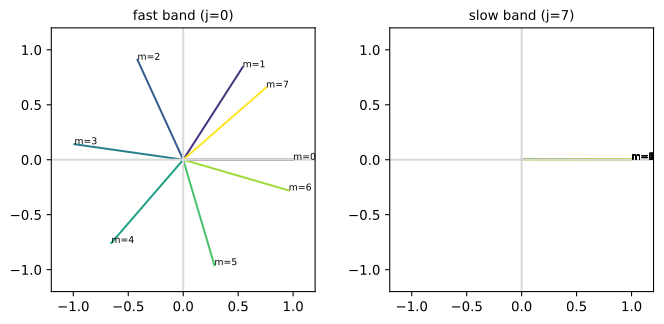
Relative dependence is not free length generalization, though. During training the model sees a bounded range of distances and phases; a low-frequency band may not complete even one rotation inside that range, so the model quietly uses it like an absolute coordinate. Push the sequence far longer at inference and those bands present phase combinations the projections never learned. Absolute offsets matter operationally too: a chunk that begins after 20,000 cached tokens must use positions starting at 20,000, or its queries rotate in a frame inconsistent with the cache — shapes still pass, retrieval quietly breaks. Position IDs are cache state.
3.6 Stretching RoPE changes the coordinate system
A model trained through context T_0 but evaluated at T_1=aT_0 needs its positions to fit the phase range it learned. RoPE extension changes the map from position to phase; it adds no training data. Position interpolation (PI) maps m\mapsto m/a, equivalently dividing every frequency by a, so positions through T_1 reuse the original phase range at the cost of compressed local resolution (Chen et al. 2023). NTK-aware scaling instead changes the base, b'=b\,a^{d_R/(d_R-2)}, which leaves the fastest band nearly untouched while stretching the slow ones. YaRN interpolates band-by-band — leaving short-wavelength bands alone, interpolating long-wavelength ones, ramping between — and also rescales the query/key magnitude to correct attention entropy (Peng et al. 2023). We build all four band constructions in one function.
# @save
import math


def ntk_base(base: float, factor: float, dim: int) -> float:
    """Return the NTK-aware adjusted RoPE base for an extension ``factor``.

    NTK-aware scaling stretches low frequencies more than high ones by raising
    the base, so local resolution survives better than under uniform
    interpolation.

    Args:
        base: The original RoPE base ``b``.
        factor: Context extension factor ``a >= 1``.
        dim: Rotary dimension ``d_R``.

    Returns:
        The adjusted base ``b'``.

    Raises:
        ValueError: If ``dim <= 2`` or ``factor < 1``.
    """
    if dim <= 2 or factor < 1:
        raise ValueError("NTK scaling requires dim > 2 and factor >= 1")
    return base * factor ** (dim / (dim - 2))


def _correction_index(rotations: float, dim: int, base: float, original: int) -> float:
    return dim * math.log(original / (rotations * 2 * math.pi)) / (2 * math.log(base))


def inverse_frequencies(dim: int, *, method: str = "rope", base: float = 10_000.0,
                        factor: float = 1.0, original_context: int = 2_048,
                        beta_fast: float = 32.0, beta_slow: float = 1.0) -> tuple[Tensor, float]:
    """Return RoPE band frequencies under a context-extension method.

    Each method reshapes the ``dim/2`` bands of @eq-ch03-rope differently:
    ``rope`` is unscaled; ``pi`` divides every band by ``factor``; ``ntk``
    raises the base so high bands survive; ``yarn`` interpolates band-by-band
    and also returns a query/key magnitude multiplier (its attention
    temperature). Only YaRN returns a magnitude other than 1.

    Args:
        dim: Rotary dimension ``d_R`` (even, >= 4).
        method: One of ``"rope"``, ``"pi"``, ``"ntk"``, ``"yarn"``.
        base: Original RoPE base ``b``.
        factor: Extension factor ``a``.
        original_context: Trained context ``T_0`` (used by YaRN's ramp).
        beta_fast, beta_slow: YaRN band boundaries in rotations per ``T_0``.

    Returns:
        A tuple ``(frequencies, magnitude)``: the ``dim/2`` band frequencies and
        the scalar applied to rotated queries and keys.

    Raises:
        ValueError: If ``dim`` is invalid or the method is unknown.
    """
    if dim % 2 or dim < 4 or factor < 1:
        raise ValueError("dim must be even and >= 4; factor must be >= 1")
    indices = torch.arange(0, dim, 2, dtype=torch.float64)
    ordinary = base ** (-indices / dim)
    method = method.casefold()
    if method == "rope":
        return ordinary, 1.0
    if method == "pi":
        return ordinary / factor, 1.0
    if method == "ntk":
        return ntk_base(base, factor, dim) ** (-indices / dim), 1.0
    if method != "yarn":
        raise ValueError(f"unknown RoPE method: {method}")
    interpolated = ordinary / factor
    low = max(math.floor(_correction_index(beta_fast, dim, base, original_context)), 0)
    high = min(math.ceil(_correction_index(beta_slow, dim, base, original_context)), dim // 2 - 1)
    high = high + 1e-3 if low == high else high
    ramp = ((torch.arange(dim // 2, dtype=torch.float64) - low) / (high - low)).clamp(0, 1)
    frequencies = interpolated * ramp + ordinary * (1 - ramp)
    magnitude = 0.1 * math.log(factor) + 1.0 if factor > 1 else 1.0
    return frequencies, magnitude
We build the four band vectors for a fourfold extension and read the distinctions the tests will pin: PI divides uniformly, NTK holds the top band fixed while shrinking the rest, and YaRN sits between the two.
rope, _ = inverse_frequencies(16)
pi, _ = inverse_frequencies(16, method="pi", factor=4)
ntk, _ = inverse_frequencies(16, method="ntk", factor=4)
yarn, mag = inverse_frequencies(16, method="yarn", factor=4, original_context=32)
print(f"top band  RoPE {rope[0]:.4f} | PI {pi[0]:.4f} | NTK {ntk[0]:.4f} | YaRN {yarn[0]:.4f}")
print(f"low band  RoPE {rope[-1]:.4f} | PI {pi[-1]:.4f} | NTK {ntk[-1]:.4f} | YaRN {yarn[-1]:.4f}")
print(f"PI == RoPE/4: {torch.allclose(pi, rope / 4)}   YaRN between PI and RoPE: "
      f"{bool((yarn >= pi).all() and (yarn <= rope).all())}   YaRN magnitude: {mag:.3f}")
top band RoPE 1.0000 | PI 0.2500 | NTK 1.0000 | YaRN 1.0000
low band RoPE 0.0003 | PI 0.0001 | NTK 0.0001 | YaRN 0.0001
PI == RoPE/4: True YaRN between PI and RoPE: True YaRN magnitude: 1.139PI shifts the whole spectrum down by four; NTK pins the top band (0.7071) and only bends the tail; YaRN’s magnitude exceeds one, its temperature correction. Figure 3.6 plots the wavelength each band covers under the four methods, which is the shape these numbers describe.
Show the code that draws this figure
fig, ax = plt.subplots(figsize=(6.6, 3.7))
idx = range(8)
for freq, name, style in [(rope, "RoPE", "k-"), (pi, "PI", "--"), (ntk, "NTK", "-."), (yarn, "YaRN", ":")]:
    ax.semilogy(idx, [2 * math.pi / f for f in freq.tolist()], style, label=name, marker="o", ms=3)
ax.set_xlabel("rotary dimension index j")
ax.set_ylabel("band wavelength (log)")
ax.legend()
fig.tight_layout()
plt.show()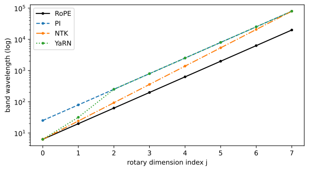
Three engineering rules follow. The extension factor is part of the model config and must match training or adaptation. A method can raise far-position quality while blurring local order, so short-context regression is a required check. And dynamic schemes whose scale tracks the current length can leave earlier and later cache entries on different maps unless keys are stored pre-rotation — cache semantics, again. ABF (a larger fixed base) and LongRoPE (searched per-band factors) extend the same idea with more tuning surface.
3.7 No position, dropped position, and distributed context
RoPE extension is not the only response to length. NoPE removes explicit position encodings entirely; the causal mask still imposes an order (position t sees t prefix states, an earlier one sees fewer), and causal Transformers without position encodings have been shown to infer usable relative signals and extrapolate surprisingly well on some tasks (Kazemnejad et al. 2023). The absence of an explicit encoding is not the absence of order, nor a guaranteed quality win. DroPE treats explicit position as a training scaffold: start from a RoPE model, remove the embeddings, and briefly recalibrate — an inductive bias that eased training becomes an extrapolation constraint later, so it is removed after the fact rather than never added.
Long context can also be a systems property. Ring Attention partitions one long sequence across devices, circulating key-value blocks around a ring while overlapping communication with blockwise attention; the global pattern stays dense, and the logical KV state is unchanged — merely divided so a sequence longer than one device’s memory fits. That is worth seeing as a number: partitioning does not shrink the cache, it spreads it.
seq = KVConfig("GQA-8", layers=32, query_heads=32, kv_heads=8, head_dim=128, bytes_per_scalar=2)
total = kv_bytes(seq, 131_072)
for devices in (1, 4, 8):
    print(f"{devices} device(s): {total / 2**30:.1f} GiB total, {total / devices / 2**30:.2f} GiB each")
1 device(s): 16.0 GiB total, 16.00 GiB each
4 device(s): 16.0 GiB total, 4.00 GiB each
8 device(s): 16.0 GiB total, 2.00 GiB eachDual Chunk Attention takes a different route, redefining rotary relations within, across, and between chunks so large global offsets stay representable without a sliding window — distant chunks remain attendable. This chapter’s decision boundary is clean: if the problem is state bytes, change head sharing, compression, or visibility; if it is position extrapolation, change or remove the coordinate mechanism with adaptation; if it is single-device capacity, partition the sequence. Chapters 6 and 10 own the distributed-training and distributed-serving mechanics.
3.8 Advertised context is not effective context
“Context window” hides three different quantities: accepted context (the largest request the runtime admits), trained context (the length distribution seen during optimization), and effective context (the positions and lengths over which a task stays above a quality bar). Only the third is a capability claim, and it is task-specific — a model can accept a huge tensor, keep finite perplexity, recover a literal passkey, and still fail to combine two facts buried in the middle. The “Lost in the Middle” study found exactly this U-shape: information near the start or end of a long context was used better than information in the middle (Liu et al. 2024), and the broader phenomenon of quality decaying as more context is added is now called context rot. There is no universal “useful fraction”; it must be measured on the deployed model and prompt.
We can isolate one cause of the shape — rotary phase — without a language model at all, using a probe that is honest about what it does and does not show. Each trial plants a content “needle” at a chosen depth among random distractor keys, rotates everything with a chosen RoPE method at a fourfold extension, and asks whether the needle wins the dot product against the end-position query.
# @save
def retrieval_probe(method: str, *, seed: int = 1_700, trials: int = 256, context: int = 128,
                    original_context: int = 32, dim: int = 32) -> list[dict[str, float]]:
    """Measure rotary retrieval versus needle depth, without a trained model.

    At each of 21 depths, ``trials`` independent trials place one content needle
    among random distractor keys, rotate keys and the end-position query with
    ``method`` at ``context / original_context`` extension, and record whether
    the needle receives the top dot product. This isolates RoPE phase effects;
    it has no learned weights, instruction hierarchy, or attention sinks, so its
    curve is a mechanism illustration, not a language-model benchmark.

    Args:
        method: A RoPE method understood by ``inverse_frequencies``.
        seed: Base seed; depth ``i`` uses ``seed + i`` for reproducibility.
        trials: Independent trials averaged per depth.
        context: Sequence length swept.
        original_context: Trained length ``T_0``; the extension factor is
            ``context / original_context``.
        dim: Rotary dimension of the probe vectors.

    Returns:
        One dict per depth with ``depth_percent``, ``accuracy``, and
        ``standard_error``.
    """
    factor = context / original_context
    freqs, magnitude = inverse_frequencies(dim, method=method, factor=factor, original_context=original_context)
    rows: list[dict[str, float]] = []
    for i, depth in enumerate(torch.linspace(0, 1, 21)):
        g = torch.Generator().manual_seed(seed + i)
        content = torch.randn(trials, dim, generator=g)
        query = content + 0.15 * torch.randn(trials, dim, generator=g)
        needle = content + 0.15 * torch.randn(trials, dim, generator=g)
        keys = torch.randn(trials, context, dim, generator=g)
        pos = round(float(depth) * (context - 2))
        keys[:, pos] = needle
        q_rot = apply_rope(query[:, None], torch.tensor([context - 1]), freqs, magnitude)[:, 0]
        k_rot = apply_rope(keys, torch.arange(context), freqs, magnitude)
        scores = torch.einsum("btd,bd->bt", k_rot, q_rot) / dim**0.5
        hits = int((scores.argmax(1) == pos).sum())
        p = hits / trials
        rows.append({"depth_percent": round(float(depth) * 100),
                     "accuracy": p, "standard_error": math.sqrt(p * (1 - p) / trials)})
    return rows
We run the probe under unscaled RoPE, NTK, and YaRN and print the mean top-1 rate for each.
runs = {m: retrieval_probe(m) for m in ("rope", "ntk", "yarn")}
for m, rows in runs.items():
    mean = sum(r["accuracy"] for r in rows) / len(rows)
    print(f"{m:5s}: mean top-1 retrieval {mean:.3f}")
rope : mean top-1 retrieval 0.600
ntk : mean top-1 retrieval 0.696
yarn : mean top-1 retrieval 0.832Unscaled RoPE recovers the needle 60% of the time on average, NTK 70%, YaRN 83% — changing only the coordinate map changes retrieval, with nothing else different. Figure 3.7 plots the full depth curves with binomial confidence bands.
Show the code that draws this figure
fig, ax = plt.subplots(figsize=(6.6, 3.7))
for (m, rows), (color, ls) in zip(runs.items(), [("#7356a8", "-"), ("#2a7f9e", "--"), ("#b13f3f", ":")]):
    xs = [r["depth_percent"] for r in rows]
    ys = [r["accuracy"] for r in rows]
    lo = [max(0, r["accuracy"] - 1.96 * r["standard_error"]) for r in rows]
    hi = [min(1, r["accuracy"] + 1.96 * r["standard_error"]) for r in rows]
    ax.plot(xs, ys, ls, color=color, label={"rope": "RoPE", "ntk": "NTK", "yarn": "YaRN"}[m])
    ax.fill_between(xs, lo, hi, color=color, alpha=0.12)
ax.set_xlabel("needle depth from start of context (%)")
ax.set_ylabel("top-1 retrieval rate")
ax.legend()
fig.tight_layout()
plt.show()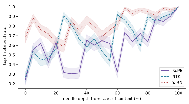
The curve isolates one mechanism; it has no trained weights and cannot show semantic lost-in-the-middle. Its value is causal: it proves the coordinate map alone moves retrieval, which is why an “effective context” claim must be measured, not inherited from a spec.
NoteIn the interview
Q. A model advertises a 1M-token window and a PM asks whether we can drop retrieval and just paste everything in. What do you check? Separate accepted from effective context: the 1M is an interface limit, not a capability guarantee. Measure effective context on your task with a length-by-depth grid (retrieval, multi-hop, aggregation), watch for context rot as distractors grow, and price the KV cache and decode latency at that length. The trap is treating the advertised number as proof of accurate use everywhere; the strong answer names the measurement — task quality stratified by length and depth — that would settle it.
3.9 Benchmark the failure you care about
A long-context benchmark is useful only when its failure mode matches your application, and the field’s suites climb a ladder of difficulty for exactly that reason. Our own probe is a Needle-in-a-Haystack (NIAH) test in miniature: a literal key planted at a controlled depth, recovered by direct match. NIAH is a great smoke test — cheap, position-controlled, and quick to expose truncation or position-ID bugs — but it saturates first, because exact lexical cues let attention match the needle directly. That is precisely the weakness the next rung removes. RULER varies length and adds multi-hop tracing and aggregation, so effective length is comparable across models (Hsieh et al. 2024). NoLiMa strips the literal overlap: the query and needle connect only through latent knowledge, so keyword matching no longer solves it (Modarressi et al. 2025). LongBench v2 moves to realistic long-document QA, code, and structured-data reasoning.
Seen this way, the probe’s content = needle + noise construction is what makes it a literal-match task; making the needle recoverable only through an alias chain (entity → alias → value, with no shared surface tokens) is exactly the step from NIAH to NoLiMa, and it demands abilities the probe has no weights for. A serious evaluation therefore records tokenizer length (not characters), evidence depth and span, distractor count, task type (literal, associative, aggregation, reasoning), an original-window regression baseline, accuracy with confidence intervals, and prefill/decode/memory cost — and does not average them into one number, because a single score hides a dead middle or a cliff just past the trained length. Chapter 22 turns this grid into a full evaluation system; Chapter 13 owns the context engineering — selection, ordering, compaction — that decides what goes into the window in the first place.
NoteLandscape 2026 — a maximum-window claim is a hypothesis
Meta’s Llama 4 announcement and Scout model card advertise a 10-million-token context window. That is a valid interface and architecture claim to test, not evidence that every task stays accurate at every depth through 10M tokens.
Verify live: inspect the current Llama 4 announcement and Scout model card, then run your target task at stratified lengths and depths before turning the number into a requirement. Verified: 2026-07-19.
3.10 Summary
Persistent attention state is B\,T\,L\,(2H_{kv}d_h)\,s — a formula we ran to turn 128K tokens into 64 GiB, then shrank three ways: sharing KV heads (GQA/MQA) cuts the ratio H_{kv}/H_q; a latent cache (MLA) compresses the stored width to r+d_R; sliding windows and interleaving bound it by \min(T,W), with attention sinks keeping windows stable. RoPE replaces absolute positions with rotations whose dot product depends only on relative offset, and PI, NTK, and YaRN reshape its frequency bands to reach past the trained length. Our own probe showed scaling moving retrieval — proof that accepted context is not effective context. Chapter 10 makes this arithmetic operational in a serving stack.
3.11 Exercises
- Audit a new configuration. Pick a current open-weight model, read L, H_q, H_{kv}, d_h, and cache dtype from its
config.json, and build aKVConfigfor it. (a) Compute batch-one KV bytes at 32K and 128K by hand, then check againstkv_bytes. (b) Which single field would you change to halve the cache, and what would you have to re-validate before trusting it? - Reach MQA by the dial. Set
kv_heads=1inGroupedQueryAttentionwhile holding width and query heads fixed. Predict the cache shape and the ratio from Equation 3.2 before running, then verify. Explain why matching output shape does not prove correctness, and which check in this chapter does. - Price a window schedule. Using the interleaving computation in Section 3.4, sweep the window W and the local:global ratio for a 128K-token GQA model. Plot cache GiB against W, and find the schedule that fits a 12 GiB budget. What long-range capability did you trade away, and which benchmark rung would catch it?
- Break the rotary frame. Modify
ToyLatentKVAttention(orGroupedQueryAttention) so that each appended chunk restarts its position counter at zero. Construct a two-chunk sequence, compare the cached output to a full pass, and plot the error by position. Explain why tensor shapes and cache bytes stay valid while attention silently degrades. - Reshape the bands yourself. Using
inverse_frequencies, extend the retrieval probe with a fifth method that divides only the slowest half of the bands. Predict where on the depth curve it should help or hurt relative to YaRN, run it, and report the mean and the depth profile. Which real method does your hand-made one most resemble? - Make the probe associative. Replace the probe’s direct
content = needle + noisewith a two-record alias chain (entity→alias, alias→value) that shares no surface tokens with the query. Report retrieval by depth, explain which part of the change pushes the probe toward NoLiMa, and name the model ability the probe still cannot exercise.